前言

使用 Tidyverse 风格书写代码主要侧重于数据分析，而非编程¹:。

更快的熟悉方式可以参考DataCamp上的这门课程 Add to Tidyverse (FREE)(Li 2018) 。

代码的书写原则

写可读的代码(王垠 2015)，不要冗长的解释，因为这实际上在增加使用者的阅读量，这是管道代码的主要优点。
尽量使用#隐去中间过程的代码，这样即省略了中间变量的设立，也让使用者理解开发者的用意
使用 pipeline 或者中间变量²，方便大家理解代码。

李家翔
于上海

作者简介

参考Stack Overflow插入。

1 magrittr 包的使用

Tidyverse 风格的代码会常使用到管道%>%，这只是其中最常见的一种。更多管道知识，参考GitHub

magrittr包的主要目标有2个 (张丹 2018)

第一是减少代码开发时间，提高代码的可读性和维护性；

第二是让你的代码更短

主要四种pipeline。

%>%
%T>%: tee operator
%$%
%<>%

我发现pipeline的功效需要举例说明，更直观。

1.1 `%>%`

参考 github

x %>% f %>% g %>% h = h(g(f(x)))
x %>% f(y, z = .) = f(y, z = x)
x %>% {f(y = nrow(.), z = ncol(.))} = f(y = nrow(x), z = ncol(x))

以下举例。

取10000个随机数符合，符合正态分布。
求这个10000个数的绝对值，同时乘以50。
把结果组成一个100*100列的方阵。
计算方阵中每行的均值，并四舍五入保留到整数。
把结果除以7求余数，并话出余数的直方图。

set.seed(1)
rnorm(n=10000) %>% 
    abs %>% 
    `*` (50) %>% 
    matrix(ncol=100) %>% 
    rowMeans %>% 
    round %>% 
    `%%` (7) %>% 
    hist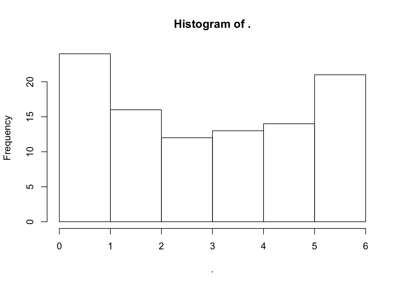

1.2 `%T>%`

取10000个随机数符合，符合正态分布。
求这个10000个数的绝对值，同时乘以50。
把结果组成一个100*100列的方阵。
计算方阵中每行的均值，并四舍五入保留到整数。
把结果除以7求余数，并话出余数的直方图。
对余数求和

set.seed(1)
rnorm(10000) %>% 
    abs %>% 
    `*` (50) %>% 
    matrix(ncol = 100) %>% 
    rowMeans %>% 
    round %>% 
    `%%` (7) %T>% 
    hist %>% 
    sum

## [1] 328

可以发现g保证了最后两个output通过

`%%` (7)

产生。

1.3 `%$%`

Many functions accept a data argument, e.g. lm and aggregate, which is very useful in a pipeline where data is first processed and then passed into such a function. There are also functions that do not have a data argument, for which it is useful to expose the variables in the data. This is done with the %$% operator. https://github.com/tidyverse/magrittr

终于理解了 $ 就是 obj$x$y。

iris %>%
  subset(Sepal.Length > mean(Sepal.Length)) %$%
  cor(Sepal.Length, Sepal.Width)
#> [1] 0.3361992

这样可以省略.$a

1.4 `%<>%`

类似于 pandas 中函数的 replace = TRUE 参数。

1.5 还可以传递函数

iris %>% 
(
function(x) {
    if(nrow(x) > 2)
        bind_rows(x %>% head(1),x %>% tail(1))
    else x
}
)

这里使用了 if ... else 函数，不会出现封装逻辑的报错，比如ifelse老是反馈向量化的结果。

2 read_* 数据

参考 jiaxiangbu 和 jiaxiangbu

2.1 `read_*`文档

Yihui 在 blogdown 包中采用read_utf8 {xfun}而非read_file，保证了代码是UTF-8录入。 read_utf8虽然不是 Tidyverse 集成包中的函数，但是很好的处理了编码的问题，建议大家使用。

2.2 专业的数据描述文档

参考 Östblom and Niehus (2018)

这里学习read_delim去阅读，有 comment 的数据集。

car_acc <- read_delim("datasets/road-accidents.csv",delim = '|',comment = "#")

通过

# 表达 comment
##### 表达标题

可以学习专业的数据描述文档。

##### LICENSE #####
# This data set is modified from the original at fivethirtyeight (https://github.com/fivethirtyeight/data/tree/master/bad-drivers)
# and it is released under CC BY 4.0 (https://creativecommons.org/licenses/by/4.0/)
##### COLUMN ABBREVIATIONS #####
# drvr_fatl_col_bmiles = Number of drivers involved in fatal collisions per billion miles (2011)
# perc_fatl_speed = Percentage Of Drivers Involved In Fatal Collisions Who Were Speeding (2009)
# perc_fatl_alcohol = Percentage Of Drivers Involved In Fatal Collisions Who Were Alcohol-Impaired (2011)
# perc_fatl_1st_time = Percentage Of Drivers Involved In Fatal Collisions Who Had Not Been Involved In Any Previous Accidents (2011)
##### DATA BEGIN #####
state|drvr_fatl_col_bmiles|perc_fatl_speed|perc_fatl_alcohol|perc_fatl_1st_time
Alabama|18.8|39|30|80

3 reprex 使用技巧

reprex 包是为了方便共享代码很好，这一章节主要介绍大家使用，以方便大家在网上提问。

3.1 常见报错

3.1.1 安装对应的包

reprex::reprex(
    ...
)

把要测试的代码写入...，这是最稳妥的方法。

> install.packages("shinyjs")
Error in install.packages : error reading from connection
> devtools::install_github("daattali/shinyjs")

shinyjs包会报错，没有安装包，用github安装。

3.2 数据引入

参考 McBain and Dervieux (2018) 。

library(tidyverse)
head(mtcars) %>% deparse()

## [1] "structure(list(mpg = c(21, 21, 22.8, 21.4, 18.7, 18.1), cyl = c(6, "   
## [2] "6, 4, 6, 8, 6), disp = c(160, 160, 108, 258, 360, 225), hp = c(110, "  
## [3] "110, 93, 110, 175, 105), drat = c(3.9, 3.9, 3.85, 3.08, 3.15, "        
## [4] "2.76), wt = c(2.62, 2.875, 2.32, 3.215, 3.44, 3.46), qsec = c(16.46, " 
## [5] "17.02, 18.61, 19.44, 17.02, 20.22), vs = c(0, 0, 1, 1, 0, 1), "        
## [6] "    am = c(1, 1, 1, 0, 0, 0), gear = c(4, 4, 4, 3, 3, 3), carb = c(4, "
## [7] "    4, 1, 1, 2, 1)), row.names = c(\"Mazda RX4\", \"Mazda RX4 Wag\", " 
## [8] "\"Datsun 710\", \"Hornet 4 Drive\", \"Hornet Sportabout\", \"Valiant\""
## [9] "), class = \"data.frame\")"

head(mtcars) %>% datapasta::tribble_paste()

## tibble::tribble(
##   ~mpg, ~cyl, ~disp, ~hp, ~drat,   ~wt, ~qsec, ~vs, ~am, ~gear, ~carb,
##     21,    6,   160, 110,   3.9,  2.62, 16.46,   0,   1,     4,     4,
##     21,    6,   160, 110,   3.9, 2.875, 17.02,   0,   1,     4,     4,
##   22.8,    4,   108,  93,  3.85,  2.32, 18.61,   1,   1,     4,     1,
##   21.4,    6,   258, 110,  3.08, 3.215, 19.44,   1,   0,     3,     1,
##   18.7,    8,   360, 175,  3.15,  3.44, 17.02,   0,   0,     3,     2,
##   18.1,    6,   225, 105,  2.76,  3.46, 20.22,   1,   0,     3,     1
##   )

deparse()解析表的结构，这个时候再复制粘贴就好，clipr::write_clip()执行。
datapasta::tribble_paste()直接发生inplace的反馈tibble格式的表格

3.3 其他更多功能

reprex_invert() = the opposite of reprex() From METACRAN
reprex_clean(), e.g. when you copy/paste from GitHub or StackOverflow From METACRAN
reprex_rescue(), when you’re dealing with copy/paste from R Console From METACRAN
reprex(..., si = TRUE), add session info in a folding style. From METACRAN

3.4 指定网站发布

“gh” for GitHub-Flavored Markdown, the default
“so” for Stack Overflow Markdown
“ds” for Discourse, e.g., community.rstudio.com.

3.5 可复现例子

根据我们电话沟通，目前你的反馈中没有加入 library(plm)，因此产生报错。比如我们想要查询 mtcars 的行数、列数、summary 情况，并且想知道执行后使用者的本地配置。

先写好需要的代码

library(dplyr)
mtcars %>% dim()
mtcars %>% summary()

然后复制 ctrl + c，再执行代码

reprex::reprex(si = TRUE)

这个时候会生成一个 html 文件

注意最下方有一个 session info 记录了当前的配置，点击后出现

这样就知道当前你的系统信息和相关包的安装情况了。

这个时候如果你的剪贴板没有被覆盖的话，在 GitHub 的一个对话框中，执行 ctrl + v，会发现有以下 html 代码，粘贴到对话框后，github 上显示的格式和截图中一致。

library(dplyr)
#> 
#> 载入程辑包：'dplyr'
#> The following objects are masked from 'package:stats':
#> 
#>     filter, lag
#> The following objects are masked from 'package:base':
#> 
#>     intersect, setdiff, setequal, union
mtcars %>% dim()
#> [1] 32 11
mtcars %>% summary()
#>       mpg             cyl             disp             hp       
#>  Min.   :10.40   Min.   :4.000   Min.   : 71.1   Min.   : 52.0  
#>  1st Qu.:15.43   1st Qu.:4.000   1st Qu.:120.8   1st Qu.: 96.5  
#>  Median :19.20   Median :6.000   Median :196.3   Median :123.0  
#>  Mean   :20.09   Mean   :6.188   Mean   :230.7   Mean   :146.7  
#>  3rd Qu.:22.80   3rd Qu.:8.000   3rd Qu.:326.0   3rd Qu.:180.0  
#>  Max.   :33.90   Max.   :8.000   Max.   :472.0   Max.   :335.0  
#>       drat             wt             qsec             vs        
#>  Min.   :2.760   Min.   :1.513   Min.   :14.50   Min.   :0.0000  
#>  1st Qu.:3.080   1st Qu.:2.581   1st Qu.:16.89   1st Qu.:0.0000  
#>  Median :3.695   Median :3.325   Median :17.71   Median :0.0000  
#>  Mean   :3.597   Mean   :3.217   Mean   :17.85   Mean   :0.4375  
#>  3rd Qu.:3.920   3rd Qu.:3.610   3rd Qu.:18.90   3rd Qu.:1.0000  
#>  Max.   :4.930   Max.   :5.424   Max.   :22.90   Max.   :1.0000  
#>        am              gear            carb      
#>  Min.   :0.0000   Min.   :3.000   Min.   :1.000  
#>  1st Qu.:0.0000   1st Qu.:3.000   1st Qu.:2.000  
#>  Median :0.0000   Median :4.000   Median :2.000  
#>  Mean   :0.4062   Mean   :3.688   Mean   :2.812  
#>  3rd Qu.:1.0000   3rd Qu.:4.000   3rd Qu.:4.000  
#>  Max.   :1.0000   Max.   :5.000   Max.   :8.000

^{Created on 2019-07-25 by the reprex package (v0.2.1)}

Session info

devtools::session_info()
#> ─ Session info ──────────────────────────────────────────────────────────
#>  setting  value                       
#>  version  R version 3.5.3 (2019-03-11)
#>  os       macOS Mojave 10.14.5        
#>  system   x86_64, darwin15.6.0        
#>  ui       X11                         
#>  language (EN)                        
#>  collate  zh_CN.UTF-8                 
#>  ctype    zh_CN.UTF-8                 
#>  tz       Asia/Shanghai               
#>  date     2019-07-25                  
#> 
#> ─ Packages ──────────────────────────────────────────────────────────────
#>  package     * version date       lib source                      
#>  assertthat    0.2.0   2017-04-11 [1] CRAN (R 3.5.0)              
#>  backports     1.1.2   2017-12-13 [1] CRAN (R 3.5.0)              
#>  callr         3.3.0   2019-07-04 [1] CRAN (R 3.5.2)              
#>  cli           1.1.0   2019-03-19 [1] CRAN (R 3.5.2)              
#>  crayon        1.3.4   2017-09-16 [1] CRAN (R 3.5.0)              
#>  desc          1.2.0   2018-05-01 [1] CRAN (R 3.5.0)              
#>  devtools      2.1.0   2019-07-06 [1] CRAN (R 3.5.2)              
#>  digest        0.6.18  2018-10-10 [1] CRAN (R 3.5.0)              
#>  dplyr       * 0.8.0.1 2019-02-15 [1] CRAN (R 3.5.2)              
#>  evaluate      0.12    2018-10-09 [1] CRAN (R 3.5.0)              
#>  fs            1.3.1   2019-05-06 [1] CRAN (R 3.5.2)              
#>  glue          1.3.1   2019-03-12 [1] CRAN (R 3.5.2)              
#>  highr         0.7     2018-06-09 [1] CRAN (R 3.5.0)              
#>  htmltools     0.3.6   2017-04-28 [1] CRAN (R 3.5.0)              
#>  knitr         1.22.8  2019-05-14 [1] Github (yihui/knitr@00ffce2)
#>  magrittr      1.5     2014-11-22 [1] CRAN (R 3.5.0)              
#>  memoise       1.1.0   2017-04-21 [1] CRAN (R 3.5.0)              
#>  pillar        1.3.1   2018-12-15 [1] CRAN (R 3.5.0)              
#>  pkgbuild      1.0.3   2019-03-20 [1] CRAN (R 3.5.2)              
#>  pkgconfig     2.0.2   2018-08-16 [1] CRAN (R 3.5.0)              
#>  pkgload       1.0.2   2018-10-29 [1] CRAN (R 3.5.0)              
#>  prettyunits   1.0.2   2015-07-13 [1] CRAN (R 3.5.0)              
#>  processx      3.4.0   2019-07-03 [1] CRAN (R 3.5.2)              
#>  ps            1.2.1   2018-11-06 [1] CRAN (R 3.5.0)              
#>  purrr         0.2.5   2018-05-29 [1] CRAN (R 3.5.0)              
#>  R6            2.3.0   2018-10-04 [1] CRAN (R 3.5.0)              
#>  Rcpp          1.0.0   2018-11-07 [1] CRAN (R 3.5.0)              
#>  remotes       2.1.0   2019-06-24 [1] CRAN (R 3.5.2)              
#>  rlang         0.3.1   2019-01-08 [1] CRAN (R 3.5.2)              
#>  rmarkdown     1.10    2018-06-11 [1] CRAN (R 3.5.0)              
#>  rprojroot     1.3-2   2018-01-03 [1] CRAN (R 3.5.0)              
#>  sessioninfo   1.1.1   2018-11-05 [1] CRAN (R 3.5.0)              
#>  stringi       1.4.3   2019-03-12 [1] CRAN (R 3.5.2)              
#>  stringr       1.4.0   2019-02-10 [1] CRAN (R 3.5.2)              
#>  testthat      2.1.1   2019-04-23 [1] CRAN (R 3.5.2)              
#>  tibble        2.1.1   2019-03-16 [1] CRAN (R 3.5.2)              
#>  tidyselect    0.2.5   2018-10-11 [1] CRAN (R 3.5.0)              
#>  usethis       1.5.0   2019-04-07 [1] CRAN (R 3.5.3)              
#>  withr         2.1.2   2018-03-15 [1] CRAN (R 3.5.0)              
#>  xfun          0.6     2019-04-02 [1] CRAN (R 3.5.2)              
#>  yaml          2.2.0   2018-07-25 [1] CRAN (R 3.5.0)              
#> 
#> [1] /Library/Frameworks/R.framework/Versions/3.5/Resources/library

会生成html文件

4 dplyr

参考 Baert (2018 a), Baert (2018 b), Baert (2018 c), Baert (2018 d)。

4.1 not: `~!`

msleep %>%
  select_if(~!is.numeric(.)) %>%
  glimpse

~ = function()
! = not，来自magrittr包的定义 (张丹 2018)

4.2 `select_*`

4.2.1 `select_all` = `rename_all`

mtcars %>% 
  select_all(toupper) %>% ## 让名字变为大写
  head

mtcars %>% 
  select_all(tolower) %>% ## 让名字变为小写
  head()

按照数据类型进行选择。

mtcars %>% 
  mutate(cyl = as.factor(cyl),hp = as.factor(hp)) %>% 
  select_if(is.factor)

4.2.2 `select_if` + aggregate function

msleep %>%
  select_if(~is.numeric(.) & mean(., na.rm=TRUE) > 10)

sum条件进行变量筛选
mean(., na.rm=TRUE) > 10
n_distinct(.) < 10

4.3 `head`, `glimpse`不需要`()`

 mtcars %>%
   head

4.4 `rowwise()`

rowwise()改变mean的方向，by row，而非by column

msleep %>%
  select(name, contains("sleep")) %>%
  rowwise() %>%
  mutate(avg = mean(c(sleep_rem, sleep_cycle)))

4.5 `str_trim`: 清洗边缘上的空格

"   aaa   " %>% str_trim

## [1] "aaa"

4.6 `na_if`让特定字符为`NA`

msleep %>%
  select(name:order) %>%
  na_if("omni")

msleep %>% 
  select(name, sleep_total) %>% 
  filter(str_detect(tolower(name), pattern = "mouse"))

str_detect比str_subset简单。

4.7 filter w/ conditions

filter(condition1, condition2) will return rows where both conditions are met.
filter(condition1, !condition2) will return all rows where condition one is true but condition 2 is not.
filter(condition1 | condition2)will return rows where condition 1 and/or condition 2 is met.
filter(xor(condition1, condition2) will return all rows where only one of the conditions is met, and not when both conditions are met.

4.7.1 `xor`: 开区间

data_frame(a = 1:100) %>% 
  filter(xor(a > 10, a < 90))

## Warning: `data_frame()` is deprecated, use `tibble()`.
## This warning is displayed once per session.

xor(a > 10, a < 90) = a > 10 & a>= 90 | a <= 10 & a < 90

4.7.2 `any_vars` & `all_vars`

msleep %>% 
  select(name:order, sleep_total, -vore) %>% 
  filter_all(any_vars(str_detect(., pattern = "Ca")))

any_vars
all_vars

批量筛选，满足一个条件，对多个col进行filter。

4.8 `add_count`/`add_tally` 所属level的数量/和

msleep %>%
    select(name:vore) %>%
    add_count(vore)
msleep %>%
    select(name:vore) %>%
    left_join(
        msleep %>%         
            group_by(vore) %>% 
            count()
        ,by='vore'
    )

This saves the combination of grouping, mutating and ungrouping again (Baert 2018 d).

Obtain count of unique combination of columns in R dataframe without eliminating the duplicate columns from the data. (Thomas 2017)

mtcars %>% 
    mutate(cyl=as.factor(cyl)) %>% 
    select(mpg,cyl) %>% 
    group_by(cyl) %>% 
    add_tally(mpg)

4.9 `slice`

msleep %>%
  slice(50:55)

head, tail加强版

5 rlang

We have come to realize that this pattern is difficult to teach and to learn because it involves a new, unfamiliar syntax and because it introduces two new programming concepts (quote and unquote) that are hard to understand intuitively. This complexity is not really justified because this pattern is overly flexible for basic programming needs. https://www.tidyverse.org/articles/2019/06/rlang-0-4-0/

说的占理。

packageVersion("rlang")

## [1] '0.4.0'

if (!packageVersion("rlang") >= "0.4.0") {
  install.packages("rlang")
}

get_n_unique <- function(df, by, columns) {
  df %>% 
      group_by({{by}}) %>% 
      summarise(
          n_unique = n_distinct({{columns}})
      )
}
get_n_unique(mtcars, cyl, mpg)

get_n_unique(mtcars, cyl, disp)

get_n_unique <- function(df, by, ...) {
  df %>% 
      group_by({{by}}) %>% 
      summarise(
          ...
      )
}
get_n_unique(
    df = mtcars,
    by = cyl,
    n_unique1 = n_distinct(hp),
    n_unique2 = n_distinct(disp)
)

6 实际、复合需求

需求文档格式 https://github.com/JiaxiangBU/picbackup/raw/master/demand_sample.xlsx

6.1 自动展示最新文档

可重复性研究的时候，需要保存每天跑的版本，因此保存文档的格式为date_*，

date表示日期，如181001表示18年10月1日保存的文档，可以是
1. .csv，用于传输数据
2. .png，用于展示图像
_*是文档的命名和类型，如_imptable.csv，表示重要性数据的表格

然后在展示的.Rmd直接引用，

可以设置

library(tidyverse)
library(lubridate)

## 
## Attaching package: 'lubridate'

## The following object is masked from 'package:base':
## 
##     date

today() %>% str_remove_all("-") %>% str_sub(3,8)

## [1] "190726"

但是有些报告，不是当天都要刷的，有时候直接refer昨日的数据，这时，就需要基于最新的文档就好了。

list.files('data') %>% str_subset('confusing_matrix.csv') %>% max

因此在data文件夹中，匹配相应的，命名和格式，如confusing_matrix.csv，然后选取最新的文档，用max函数实现。

不需要每天刷。

6.2 Frequency table

# df1 <- 
mtcars %>%
    dplyr::count(cyl, am) %>%
    mutate(prop = prop.table(n)) %T>%
    print %>% 
    select(-n) %>%
    # margin table
    group_by(cyl) %>% 
    mutate(prop = prop/sum(prop)) %>% 
    spread(am,prop)

## # A tibble: 6 x 4
##     cyl    am     n   prop
##   <dbl> <dbl> <int>  <dbl>
## 1     4     0     3 0.0938
## 2     4     1     8 0.25  
## 3     6     0     4 0.125 
## 4     6     1     3 0.0938
## 5     8     0    12 0.375 
## 6     8     1     2 0.0625

参考 Aizkalns (2018) 注意这里，group_by(cyl)是因为要标准化每个cyl的level的概率。

6.3 按照箱型图的逻辑，剔除outliers

remove_outliers <- function(x, na.rm = TRUE, ...) {
  qnt <- quantile(x, probs=c(.25, .75), na.rm = na.rm, ...)
  H <- 1.5 * IQR(x, na.rm = na.rm)
  y <- x
  y[x < (qnt[1] - H)] <- NA
  y[x > (qnt[2] + H)] <- NA
  y
}

Blagotić (2011) 根据箱型图定义构建函数。但是 Win. (2011) 利用函数boxplot.stats给出了更简单的方式，日后采用。

remove_outliers <- 
    function(x,comp=1.5){
    x %>% 
        boxplot.stats(.,coef = comp) %>% 
        .$out %>% 
        setdiff(x,.)    
    }

6.4 按照唯一值分bin

quantile(unique(...)) (Elferts 2013) 完成。

set.seed(123)
a <- c(rep(1,10),rep(2,10),runif(10,3,10))
breaks <- 
    a %>% 
    unique %>% 
    c(-Inf,.,Inf) %>% 
    quantile(c(0, 0.25,0.5,0.75,1))

cut(
    a
    ,breaks
)

##  [1] (-Inf,3.74] (-Inf,3.74] (-Inf,3.74] (-Inf,3.74]
##  [5] (-Inf,3.74] (-Inf,3.74] (-Inf,3.74] (-Inf,3.74]
##  [9] (-Inf,3.74] (-Inf,3.74] (-Inf,3.74] (-Inf,3.74]
## [13] (-Inf,3.74] (-Inf,3.74] (-Inf,3.74] (-Inf,3.74]
## [17] (-Inf,3.74] (-Inf,3.74] (-Inf,3.74] (-Inf,3.74]
## [21] (3.74,6.45] (6.45,9.02] (3.74,6.45] (9.02, Inf]
## [25] (9.02, Inf] (-Inf,3.74] (6.45,9.02] (9.02, Inf]
## [29] (6.45,9.02] (3.74,6.45]
## 4 Levels: (-Inf,3.74] (3.74,6.45] ... (9.02, Inf]

a %>% 
    (
        function(x)
            cut(x
                ,x %>% 
                    unique %>% 
                c(-Inf,.,Inf) %>% 
                quantile(c(0, 0.25,0.5,0.75,1))
                    )
    )

##  [1] (-Inf,3.74] (-Inf,3.74] (-Inf,3.74] (-Inf,3.74]
##  [5] (-Inf,3.74] (-Inf,3.74] (-Inf,3.74] (-Inf,3.74]
##  [9] (-Inf,3.74] (-Inf,3.74] (-Inf,3.74] (-Inf,3.74]
## [13] (-Inf,3.74] (-Inf,3.74] (-Inf,3.74] (-Inf,3.74]
## [17] (-Inf,3.74] (-Inf,3.74] (-Inf,3.74] (-Inf,3.74]
## [21] (3.74,6.45] (6.45,9.02] (3.74,6.45] (9.02, Inf]
## [25] (9.02, Inf] (-Inf,3.74] (6.45,9.02] (9.02, Inf]
## [29] (6.45,9.02] (3.74,6.45]
## 4 Levels: (-Inf,3.74] (3.74,6.45] ... (9.02, Inf]

这里function(x)参考 1.5

6.5 变量切bin分类

使用cut而非case_when

a %>% 
    cut(.,breaks = c(-Inf,0.5,2.5,Inf))

##  [1] (0.5,2.5]  (0.5,2.5]  (0.5,2.5]  (0.5,2.5] 
##  [5] (0.5,2.5]  (0.5,2.5]  (0.5,2.5]  (0.5,2.5] 
##  [9] (0.5,2.5]  (0.5,2.5]  (0.5,2.5]  (0.5,2.5] 
## [13] (0.5,2.5]  (0.5,2.5]  (0.5,2.5]  (0.5,2.5] 
## [17] (0.5,2.5]  (0.5,2.5]  (0.5,2.5]  (0.5,2.5] 
## [21] (2.5, Inf] (2.5, Inf] (2.5, Inf] (2.5, Inf]
## [25] (2.5, Inf] (2.5, Inf] (2.5, Inf] (2.5, Inf]
## [29] (2.5, Inf] (2.5, Inf]
## Levels: (-Inf,0.5] (0.5,2.5] (2.5, Inf]

这里只想切0.5,2.5

6.6 连续变量和分类变量的批量处理

我们需要

当变量为连续变量时，汇总为均值；
当变量为分类变量时，汇总为众数；

mtcars %>% 
  mutate(cyl = as.factor(cyl)) %>% 
  summarise_all(
    function(x){ifelse(is.numeric(x),mean(x),names(sort(-table(x)))[1])}
  )

6.7 众数求解

library(formattable)
mtcars %>% 
    .$cyl %>% 
    table %>% 
    sort(.,decreasing = T) %>% 
    print %>% 
    `/` (sum(.)) %>% 
    percent %>% 
    print %>% 
    head(1) %>% 
    names()

## .
##  8  4  6 
## 14 11  7 
## .
##   8   4   6 
## 44% 34% 22%

## [1] "8"

6.8 计算餐补次数

INPUT

library(data.table)

## 
## Attaching package: 'data.table'

## The following objects are masked from 'package:lubridate':
## 
##     hour, isoweek, mday, minute, month, quarter,
##     second, wday, week, yday, year

## The following objects are masked from 'package:dplyr':
## 
##     between, first, last

## The following object is masked from 'package:purrr':
## 
##     transpose

library(tidyverse)
library(lubridate)
fread("id   X1  X2
1   09:12  17:16    09:10  14:14  17:21  
2   09:54  20:24    09:54  
")

OUTPUT

fread("id   餐补次数    餐补金额
1   0   0
2   1   20
")

STEP

拆分每个人每天的上下班打卡时间（X1、X2是工作日，id是人）
分别计算每人每天的打卡时间差（每个单元格内的最大值减去最小值）
重塑一列餐补次数和餐补金额餐补次数（每人在所有工作日的餐补次数）的逻辑：最早打卡时间必须是10:10分（包括10:10分）之前，且最晚的打卡时间必须是20点（包括20点）之后，并且工作时长满足10小时（包括10）以上餐补金额就是餐补次数*20"

注：正常的给予餐补的时间是早10-晚20点，如果某人早上11点过来，晚上24点打卡，也不给餐补

fread("id   X1  X2
1   09:12  17:16    09:10  14:14  17:21  
2   09:54  20:24    09:54  
") %>% 
    mutate_if(is.character,str_squish) %>% 
    # 剔除多余空格
    mutate_if(is.character,~str_split(.,' ')) %>% 
    gather(key,value,-id) %>% 
    unnest() %>% 
    group_by(id,key) %>% 
    summarise(max=max(value),
              min=min(value)) %>% 
    # 求上班和下班时间
    mutate(
        cnt = 
            ifelse(
                (max>'20:00'
                 & min<'10:10'
                 & as.difftime(str_c(max,':00'))-as.difftime(str_c(min,':00')) > 10
                 )
                ,1,0
    )
    ) %>% 
    # 统计餐补次数
    select(id,cnt) %>% 
    group_by(id) %>% 
    summarise(cnt=sum(cnt)) %>% 
    mutate(amt = cnt*20) %>% 
    # 统计餐补金额
    set_names(c('id','餐补次数','餐补金额'))

6.9 支付宝交易记录探查

library(data.table)
library(lubridate)
'alipay_record_20181022_1240_1.csv' %>% 
    fread %>% 
    mutate(`付款时间` = ymd_hms(`付款时间`)) %>% 
    # distinct(`类型`)
    # filter(`类型` != '支付宝担保交易'
    #        ,`收/支`=='支出') %>%
    # filter(
    #     `金额（元）` < 300
    #     ,`金额（元）` > 100
    # ) %>%
    # distinct(`交易对方`)
    # names
    filter(`交易对方` %in% str_subset(`交易对方`,'寿司|拉面'))

支付宝交易记录，用fread可以直接把列表读出，不需要做处理。

7 未整理

7.1 提取分类变量名称

diamonds %>% 
  summarise_all(is.numeric) %>% 
  gather() %>% 
  filter(value == FALSE)

diamonds %>% 
  select_if(is.numeric)

7.2 求colMeans using dplyr

library(tidyverse)
rm(list = ls())
a1<-letters[1:10]
b1<-rnorm(10)
b2<-b3<-rnorm(10)
d1<-data.frame(a1,b1,b2,b3)
d1[9,3]<-NA

d1$b4<-NA

d1 %>% 
  ## mutate(new = rowMeans(. %>% select(b1,b2),
  ##                      na.rm = T))
  ## 不行，这里直接用.不能 %>% pipeline不支持
  mutate(new = rowMeans(.[,c("b1","b2")],
                       na.rm = T))

d1 %>% 
  rowwise() %>% 
  mutate(b5 = mean(c(b1,b2),na.rm = T))

rowwise不是很理解。

7.3 `->`

相当于你写了一大串%>% 最后弄完了，建立一个新表，但是不必跑回前面，写。。666

7.4 multiple left joins

How to perform multiple left joins using dplyr in R - Stack Overflow

library(plyr)

## -----------------------------------------------------

## You have loaded plyr after dplyr - this is likely to cause problems.
## If you need functions from both plyr and dplyr, please load plyr first, then dplyr:
## library(plyr); library(dplyr)

## -----------------------------------------------------

## 
## Attaching package: 'plyr'

## The following object is masked from 'package:lubridate':
## 
##     here

## The following objects are masked from 'package:dplyr':
## 
##     arrange, count, desc, failwith, id, mutate,
##     rename, summarise, summarize

## The following object is masked from 'package:purrr':
## 
##     compact

a <- 1:100
x <- data_frame(a = a, b = rnorm(100))
y <- data_frame(a = a, b = rnorm(100))
z <- data_frame(a = a, b = rnorm(100))
join_all(list(x,y,z), by='a', type='left')

也可以使用reduce函数完成，详见reduce 多表合并。

7.5 为什么`select`函数失效？

detach(package:MASS) MASS老是抢select 应该tab下这个变量看看是引用哪个包。

7.6 多重复抽样

sample(x, size, replace = FALSE, prob = NULL)

replace=F,表示不重复抽样，replace=T 表示可以重复抽样。

7.7 `xlsx::write.xlsx`导出`.xlsx`文件

xlsx::write.xlsx(mtcars, "mtcars.xlsx")

成功了，并且第一列，也就是excel中的A列，是data.frame的index。

Quick-R: Exporting Data

openxlsx::write.xlsx一直是bug。

7.7.1 `openxlsx::write.xlsx`失败分析

Error: zipping up workbook failed. Please make sure Rtools is installed or a zip application is available to R. Try installr::install.rtools() on Windows. If the "Rtools\bin" directory does not appear in Sys.getenv("PATH") please add it to the system PATH or set this within the R session with Sys.setenv("R_ZIPCMD" = "path/to/zip.exe")

7.7.1.1 1st `installr::install.rtools()`

installr::install.rtools()

7.7.1.2 Sys.getenv(“PATH”)

Sys.getenv("PATH")

7.7.1.3 Sys.setenv(“R_ZIPCMD” = “path/to/zip.exe”)

Sys.setenv("R_ZIPCMD" = "path/to/zip.exe")

openxlsx::write.xlsx doesn’t work. · Issue #1736 · r-lib/devtools

7.7.2 其他方式

dataframes2xls::write.xls(mtcars,"mtcars.xls")

这个需要Python的支持。

XLConnect::createSheet(mtcars, name = "CO2")

Error: loadNamespace()里算'rJava'时.onLoad失败了，详细内容：
  调用: fun(libname, pkgname)
  错误: JAVA_HOME cannot be determined from the Registry

7.8 批量读取文件、进行bind_rows, full join

library(tidyverse)
library(readxl)
path_tree <- file.path(dirname(getwd()),"lijiaxiang","170922 team","xiaosong2","prep")
paths <- list.files(path = path_tree, recursive = T, full.names = T)

file.path用于设计路径，方便mac和win7的R交互。 list.files生成路径的list文件，方便for循环。

xiaosong <- plyr::join_all(
  list(
  paths %>% str_subset("#1/") %>% as_tibble() %>% 
  mutate(table = map(value,read_excel)) %>% 
  .$table %>% 
  bind_rows()
  ,
  paths %>% str_subset("#10/") %>% as_tibble() %>% 
  mutate(table = map(value,read_excel)) %>% 
  .$table %>% 
  bind_rows()
  ),
  by = "采样时间",
  type = "full"
)

这个地方是重点，paths中有两类文件#1和#10，

需要先列合并，bind_rows，
再进行full join，通过key"采样时间"。

先对#1的文件路径进行处理。

paths %>% str_subset("#1/")表示只取用#1的文件路径，建立list，
as_tibble()建立为表格，列名为value，
mutate(table = map(value,read_excel))建立一个新的列，叫做table，对value的每个对象，进行，read_excel函数，相当于for循环。
提取这一列，使用.$table，这是个list
bind_rows()表示列合并这一列。

同样的对#10进行重复操作。

最后使用plyr::join_all将两个表格full join。

以下是查缺失值情况。

anyNA(xiaosong)
xiaosong %>% 
  gather() %>% 
  group_by(key) %>% 
  summarise(sum(is.na(value)))

7.9 选出每个组top几的rows

group_by()和top_n(几, 什么变量)可以选出每个组top几的rows，最后别忘了ungroup()。

7.10 批量fill

R: fill down multiple columns - Stack Overflow

fill_(df, names(df))和 fill(df, everything()) 两种都可以。 ## 查看table所有变量的缺失情况

r - Using dplyr summarise_each() with is.na() - Stack Overflow summarise_each(funs(sum(is.na(.)) / length(.))) 。

7.11 `read_excel`批量合成表

参考:

path <- "40ctdata_resave.xlsx"
cb_data <- path %>%
  excel_sheets() %>%
  set_names() %>%
  map_df(~ read_excel(path = path, sheet = .x, range = "A4:T33",
                      col_types = rep("text",20)), .id = "sheet") %>%
  write_csv("cb_data.csv")
print(cb_data, n = Inf)

我查看了，每个表格，有效行数为29行，20列。然后你可以使用数据透视表，先看均值查验各个变量。 1160= 1160行，这是合并的结果。

excel_sheets可以反馈xlsx的sheet列表。

7.12 mutate add mutiple lag variable

library(data.table)
full_data_ipt_miss_wo_scale_lag_y_15 <- 
full_data_ipt_miss_wo_scale %>% 
   ungroup() %>% 
   group_by(code) %>% 
   do(data.frame(., setNames(shift(.$return, 1:15), paste("return_lag_",seq(1:15)))))

setNames可以正对多个变量进行操作

full_data_ipt_miss_wo_scale_lag_y_15 %>% 
  select(contains("return")) %>% 
  summarise_all(funs(sum(is.na(.))))

7.12.1 参考

7.13 `select`+`matches` 正则化

Regex within dplyr/select helpers - tidyverse - RStudio Community 注意是matches ## set operation
set operation in dplyr 多了setequal，且可以对table操作。

union是并集， union_all是合并，有重复。

mtcars$model <- rownames(mtcars)
first <- mtcars[1:20, ]
second <- mtcars[10:32, ]

intersect(first, second)

union(first, second)

## [[1]]
##  [1] 21.0 21.0 22.8 21.4 18.7 18.1 14.3 24.4 22.8 19.2
## [11] 17.8 16.4 17.3 15.2 10.4 10.4 14.7 32.4 30.4 33.9
## 
## [[2]]
##  [1] 6 6 4 6 8 6 8 4 4 6 6 8 8 8 8 8 8 4 4 4
## 
## [[3]]
##  [1] 160.0 160.0 108.0 258.0 360.0 225.0 360.0 146.7
##  [9] 140.8 167.6 167.6 275.8 275.8 275.8 472.0 460.0
## [17] 440.0  78.7  75.7  71.1
## 
## [[4]]
##  [1] 110 110  93 110 175 105 245  62  95 123 123 180
## [13] 180 180 205 215 230  66  52  65
## 
## [[5]]
##  [1] 3.90 3.90 3.85 3.08 3.15 2.76 3.21 3.69 3.92 3.92
## [11] 3.92 3.07 3.07 3.07 2.93 3.00 3.23 4.08 4.93 4.22
## 
## [[6]]
##  [1] 2.620 2.875 2.320 3.215 3.440 3.460 3.570 3.190
##  [9] 3.150 3.440 3.440 4.070 3.730 3.780 5.250 5.424
## [17] 5.345 2.200 1.615 1.835
## 
## [[7]]
##  [1] 16.46 17.02 18.61 19.44 17.02 20.22 15.84 20.00
##  [9] 22.90 18.30 18.90 17.40 17.60 18.00 17.98 17.82
## [17] 17.42 19.47 18.52 19.90
## 
## [[8]]
##  [1] 0 0 1 1 0 1 0 1 1 1 1 0 0 0 0 0 0 1 1 1
## 
## [[9]]
##  [1] 1 1 1 0 0 0 0 0 0 0 0 0 0 0 0 0 0 1 1 1
## 
## [[10]]
##  [1] 4 4 4 3 3 3 3 4 4 4 4 3 3 3 3 3 3 4 4 4
## 
## [[11]]
##  [1] 4 4 1 1 2 1 4 2 2 4 4 3 3 3 4 4 4 1 2 1
## 
## [[12]]
##  [1] "Mazda RX4"           "Mazda RX4 Wag"      
##  [3] "Datsun 710"          "Hornet 4 Drive"     
##  [5] "Hornet Sportabout"   "Valiant"            
##  [7] "Duster 360"          "Merc 240D"          
##  [9] "Merc 230"            "Merc 280"           
## [11] "Merc 280C"           "Merc 450SE"         
## [13] "Merc 450SL"          "Merc 450SLC"        
## [15] "Cadillac Fleetwood"  "Lincoln Continental"
## [17] "Chrysler Imperial"   "Fiat 128"           
## [19] "Honda Civic"         "Toyota Corolla"     
## 
## [[13]]
##  [1] 19.2 17.8 16.4 17.3 15.2 10.4 10.4 14.7 32.4 30.4
## [11] 33.9 21.5 15.5 15.2 13.3 19.2 27.3 26.0 30.4 15.8
## [21] 19.7 15.0 21.4
## 
## [[14]]
##  [1] 6 6 8 8 8 8 8 8 4 4 4 4 8 8 8 8 4 4 4 8 6 8 4
## 
## [[15]]
##  [1] 167.6 167.6 275.8 275.8 275.8 472.0 460.0 440.0
##  [9]  78.7  75.7  71.1 120.1 318.0 304.0 350.0 400.0
## [17]  79.0 120.3  95.1 351.0 145.0 301.0 121.0
## 
## [[16]]
##  [1] 123 123 180 180 180 205 215 230  66  52  65  97
## [13] 150 150 245 175  66  91 113 264 175 335 109
## 
## [[17]]
##  [1] 3.92 3.92 3.07 3.07 3.07 2.93 3.00 3.23 4.08 4.93
## [11] 4.22 3.70 2.76 3.15 3.73 3.08 4.08 4.43 3.77 4.22
## [21] 3.62 3.54 4.11
## 
## [[18]]
##  [1] 3.440 3.440 4.070 3.730 3.780 5.250 5.424 5.345
##  [9] 2.200 1.615 1.835 2.465 3.520 3.435 3.840 3.845
## [17] 1.935 2.140 1.513 3.170 2.770 3.570 2.780
## 
## [[19]]
##  [1] 18.30 18.90 17.40 17.60 18.00 17.98 17.82 17.42
##  [9] 19.47 18.52 19.90 20.01 16.87 17.30 15.41 17.05
## [17] 18.90 16.70 16.90 14.50 15.50 14.60 18.60
## 
## [[20]]
##  [1] 1 1 0 0 0 0 0 0 1 1 1 1 0 0 0 0 1 0 1 0 0 0 1
## 
## [[21]]
##  [1] 0 0 0 0 0 0 0 0 1 1 1 0 0 0 0 0 1 1 1 1 1 1 1
## 
## [[22]]
##  [1] 4 4 3 3 3 3 3 3 4 4 4 3 3 3 3 3 4 5 5 5 5 5 4
## 
## [[23]]
##  [1] 4 4 3 3 3 4 4 4 1 2 1 1 2 2 4 2 1 2 2 4 6 8 2
## 
## [[24]]
##  [1] "Merc 280"            "Merc 280C"          
##  [3] "Merc 450SE"          "Merc 450SL"         
##  [5] "Merc 450SLC"         "Cadillac Fleetwood" 
##  [7] "Lincoln Continental" "Chrysler Imperial"  
##  [9] "Fiat 128"            "Honda Civic"        
## [11] "Toyota Corolla"      "Toyota Corona"      
## [13] "Dodge Challenger"    "AMC Javelin"        
## [15] "Camaro Z28"          "Pontiac Firebird"   
## [17] "Fiat X1-9"           "Porsche 914-2"      
## [19] "Lotus Europa"        "Ford Pantera L"     
## [21] "Ferrari Dino"        "Maserati Bora"      
## [23] "Volvo 142E"

setdiff(first, second)

setdiff(second, first)

union_all(first, second)

setequal(mtcars, mtcars[32:1, ])

## [1] TRUE

## 就是行重排列

7.14 `dplyr::select_vars`

suppressMessages(library(tidyverse))
# select_vars(names(mtcars),contains("p"))
names(mtcars) %>% str_subset("p")

## [1] "mpg"  "disp" "hp"

参考:

gather_ no longer supports dropping a column? · Issue #109 · tidyverse/tidyr

7.15 DataProfile

DataProfile

library(tidyverse)

mtcars[2,2] <- NA ## Add a null to test completeness

DataProfile <- mtcars %>%
  summarise_all(funs("Total" = n(),
                     "Nulls" = sum(is.na(.)),
                     "Filled" = sum(!is.na(.)),
                     "Cardinality" = length(unique(.)))) %>%
  reshape2::melt() %>%
  separate(variable, into = c('variable', 'measure'), sep="_") %>%
  spread(measure, value)  %>%
  mutate(Complete = Filled/Total,
         Uniqueness = Cardinality/Total,
         Distinctness = Cardinality/Filled)

## Warning: funs() is soft deprecated as of dplyr 0.8.0
## please use list() instead
## 
## # Before:
## funs(name = f(.)
## 
## # After: 
## list(name = ~f(.))
## This warning is displayed once per session.

## No id variables; using all as measure variables

DataProfile

7.16 `column_to_rownames`

mtcars %>%
  rownames_to_column() %>%
  as.data.frame() %>%
  column_to_rownames()

之前要加as.data.frame()

has_rownames(df)

remove_rownames(df)

rownames_to_column(df, var = "rowname")

rowid_to_column(df, var = "rowid")

column_to_rownames(df, var = "rowname")

7.17 transpose 函数

必须设计好index

mtcars %>% t() %>% as.data.frame()

7.18 `split`批量展示

bind_cols(imp10_vars_w_lag_15,imp10_vars_w_lag_15_partition_index) %>% 
  select(index,everything()) %>% 
  split(.$index)

7.19 这是gather最标准的写法，不会报错

gather_(key_col = "key",value_col = "value", gather_cols = x_list)

7.20 `%>%`下正则化修改变量名称

df <- df %>%
  rename_all(
      funs(
        stringr::str_to_lower(.) %>%
        stringr::str_replace_all(., '\\.', '_')
      )
  )

注意，stringr的函数需要%>%连接 (Marthe 2015)。

7.21 `lag`和`diff`的取舍

Error in mutate_impl(.data, dots) : Column daily_return must be length 488 (the group size) or one, not 487的报错。最简单的改进就是加入c(NA,diff(close))(sasikala appukuttan 2016)，因为这里少了一个单元格，第一个diff是计算不出来的，因此加入就好。或者用lag，因为会直接产生NA(Lemm 2015)，不报错。因此两个都可以用，但是要注意适用条件。

7.22 rename in pipeline

iris2 <- data.frame(iris)
iris2 %>% 
data.table::setnames(
    old = "Petal.Length",
    new = "petal_length") %>% 
    head
iris2 %>% 
    head
iris %>% 
    head

推荐purrr::set_names函数 (Rodrigues 2017)。因为data.table::setnames有inplace的功能，不适用于重复性研究。如上面的例子，iris2是iris是一个复制后data.frame，详见7.23，但是一旦进行了data.table::setnames的修改后，iris2的命名就会永久修改。

或者使用

`colnames<-`("...")

注意中间没有空格。

tibble(c(1, 2)) %>% 
    `colnames<-`("returns")

7.22.1 `make.names`的效果

make.names(c("a and b", "a-and-b"), unique = TRUE)

## [1] "a.and.b"   "a.and.b.1"

7.23 复制一个`data.frame`

<-还是会传递修改情况的。
<- data.frame()完成复制一个data.frame(Stack Overflow 2017)

7.24 `case_when`和`str_detect`的使用

library(tidyverse)

files_name <- list.files(file.path(getwd(),"wg"), full.names = T)

files_name_a <- files_name %>% str_subset("a_")
files_name_b <- files_name %>% str_subset("b_")

all_data_a <-
  files_name_a %>%
  as_tibble() %>%
  mutate(table = map(files_name_a, read_csv)) %>%
  .[-1] %>%
  unnest()

all_data_b <-
  files_name_b %>%
  as_tibble() %>%
  mutate(table = map(files_name_b, read_csv)) %>%
  .[-1] %>%
  unnest()

setwd函数最好别用，比较干扰读者的路径。这个讨论在RStudio Community上面讨论很多， Bryan (2017) 开发了一个 here 包，专门来针对这个问题，但是我觉得不是特别有效，所以没用。尽量使用file.path来设置路径就好了。

files_name %>%
  as_tibble() %>%
  mutate(
    table = map(value, read_csv),
    tag =
      case_when(
        str_detect(value,"a_") ~ "a",
        str_detect(value,"b_") ~ "b"
      )
  ) %>%
  unnest()

这里可以简化用case_when和str_detect完成，最后按需用filter函数来分表。 (Wade 2018)

7.25 dplyr中的set operation

dplyr::setequal(x, y, ...)会反馈两表的不同之处，例如 FALSE: Cols in y but not x: X1.，意思是表x中不含有表y中的X1列。这个时候再用setdiff分别进行

setdiff(x,y)
setdiff(y,x)

7.26 cumany 和 cumall 函数

tibble(a = c(8,1,2,5,6,3,4,7)) %>% filter(a > 3)

tibble(a = c(8,1,2,5,6,3,4,7)) %>% filter(cumany(a > 3))

tibble(a = c(8,1,2,5,6,3,4,7)) %>% filter(cumall(a > 3))

cumany()反馈只要之前满足条件，就会保留记录。因此三种情况中，这种情况保留的记录最多。(Wickham et al. 2018)
相反，cumall()反馈之前需要全部满足条件，才会保留记录。因此三种情况中，这种情况保留的记录最少。

7.27 Window functions

参考 Wickham et al. (2018)

7.27.1 Ranking functions

7.27.1.1 dplyr

tibble(
  x = c(1, 1, 2, 2, 2, NA)
) %>%
  mutate(
    row_number = row_number(x),
    min_rank = min_rank(x),
    dense_rank = dense_rank(x),
    dense_rank_desc = dense_rank(desc(x))
  )

7.27.1.2 impala 中的表现

with tbl_1 as
(
  select 1 as x union all
  select 1 as x union all
  select 2 as x union all
  select null as x union all
  select null as x union all
  select null as x union all
  select 2 as x union all
  select 2 as x
)
select x,
  row_number() over(order by x) as x_r_no
from tbl_1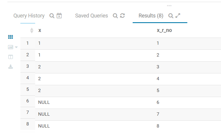

with tbl_1 as
(
  select 1 as x union all
  select 1 as x union all
  select 2 as x union all
  select null as x union all
  select null as x union all
  select null as x union all
  select 2 as x union all
  select 2 as x
)
select x,
  row_number() over(order by x desc) as x_r_no
from tbl_1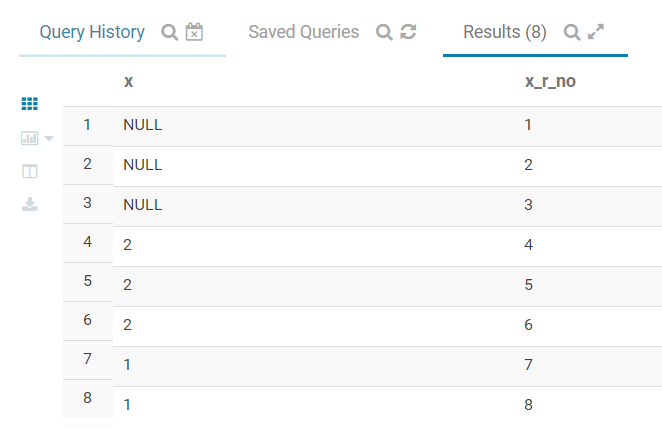

在impala里面NULL默认为最大，和Python Pandas 包的设计相同。但是和R dplyr 包的设定不同。

7.27.1.3 Pandas

参考 The pandas project (2017) 的 rank函数中的两种 method，first 和 min。

print pd.concat([z,pd.DataFrame({'x': [np.nan],'y': 7})]).x.rank(method='first', ascending=True)
print pd.concat([z,pd.DataFrame({'x': [np.nan],'y': 7})]).x.rank(method='first', ascending=False)
print pd.concat([z,pd.DataFrame({'x': [np.nan],'y': 7})]).x.rank(method='min')

0    1.0
1    2.0
2    3.0
0    NaN
Name: x, dtype: float64
0    3.0
1    2.0
2    1.0
0    NaN
Name: x, dtype: float64
0    1.0
1    2.0
2    3.0
0    NaN
Name: x, dtype: float64

dplyr 包在 ranking 函数中进行了解释。

row_number(): equivalent to rank(ties.method = "first")
min_rank(): equivalent to rank(ties.method = "min")

7.27.1.4 总结

Pandas 和 dplyr 对空值不排序和打分。然而 impala 默认 null 最大。

7.27.1.5 累计百分比

library(formattable)
x <- c(1, 1, 2, 2, 2, NA)
x

## [1]  1  1  2  2  2 NA

cume_dist(x) %>% percent()

## [1] 40.00%  40.00%  100.00% 100.00% 100.00%  NA

percent_rank(x) %>% percent()

## [1] 0.00%  0.00%  50.00% 50.00% 50.00%  NA

7.27.1.5.1 cume_dist

这个类似于SQL中 top n % 的函数。

... %>%
  filter(cume_dist(desc(x)) < 0.1)

7.27.1.5.2 ntile()

类似于ggplot2::cut_number函数，这里做一定的比较。

diamonds %>%
  select(carat) %>%
  mutate(
    grp_1 = cut_number(carat, 10),
    grp_2 = ntile(carat, 10),
    grp_3 = as.integer(grp_1)
  )

因此这里可以说几个ntile的优点

ntile 省略重命名group，省略as.integer(grp_1)这一步
而且不需要面对难看的开闭区间，就算需要知道切分点，直接用quantile 函数不是更好吗？(使用summarise函数)

7.27.1.5.3 floor 函数

简单来说就是找到第四列的最大值，然后建立从0到max值的区间，区间间隔为5000000但最后的区间结尾应该是最大值。

这个的实现就是floor和ggplot2::cut_*函数就可以了，这里使用cut_width函数。

floor函数用于向上取整，比如floor(a*5)/5就是按照5个单位向上取整。
cut_width函数控制区间长度。(Brandl 2017)
as.character、str_remove_all和separate函数主要是把得到的区间文本化，提取区间上下限制。

library(tidyverse)
# library(kable)
# library(kableExtra)
data_frame(
    x = c(rep(44,10),rep(67,10),rep(101,10))
) %>% 
    mutate(x_cut = cut_width(floor(x),50)) %>% 
    mutate(x_cut = as.character(x_cut)) %>% 
    mutate(x_cut = str_remove_all(x_cut,"\\[|\\]")) %>% 
    separate(x_cut,into = c('left','right'),sep=',')

    # kable("html") %>% 
    # kable_styling() %>% 
    # column_spec(2:3,bold = T)

7.27.2 Lead and lag

x <- 1:5
lead(x)

## [1]  2  3  4  5 NA

lag(x)

## [1] NA  1  2  3  4

x - lag(x)

## [1] NA  1  1  1  1

diff(x)

## [1] 1 1 1 1

c(NA,diff(x))

## [1] NA  1  1  1  1

x - lag(x)和c(NA,diff(x))才等价。

7.28 arrange 搭配复合条件

file.path(
  getwd() %>% dirname(),
  "fcontest",
  "xiaosong_sent_files",
  "cor_end.csv"
) %>%
  read_csv() %>%
  mutate_if(is.double, percent) %>%
  gather(key,value,-colnames) %>%
  arrange(desc(abs(value)))

一种简单写法desc(abs(value))

7.29 自定义虚拟化

data.table::data.table(
    a = c(
        rep(0,100),
        rnorm(1000, mean = 10, sd = 10)
    )
) %>%
    # filter(a >= 0) %>%
    # ggplot(aes(x = a)) +
    # geom_freqpoly()
    mutate(b = case_when(
        a == 0 ~ "0",
        a > 0 ~ as.character(ntile(a,4))
    )) %>%
    .$b %>%
    table()

## .
##   0   1   2   3   4 
## 100  13 275 275 275

7.30 json格式文件清理成dataframe

library(tidyverse)
library(rjson)
json_file_path <- file.path(getwd(),"deployment","20180525175742.txt")
json_file_tbl <- readLines(json_file_path) %>% as.data.frame()
names(json_file_tbl) <- "raw"

json_file_path: 写入json文件的路径，可以是超链接也可以是本地连接
readLines和as.data.frame()将json格式的文档，转化成dataframe格式

json_file_tbl %>%
    mutate(raw = paste("[",raw,"]", sep="")) %>%
    mutate(raw = map(.x = raw,.f = jsonlite::fromJSON)) %>%
    unnest() %>%
    gather(key = "userid") %>%
    filter(!is.na(value)) %>%
    mutate(raw = map(.x = value,.f = jsonlite::fromJSON)) %>%
    select(-value) %>%
    unnest() %>%
    group_by(userid) %>%o
    mutate(No = 1:n()) %>%
    write_csv(file.path(getwd(),"deployment","data","json_file_to_df.csv")) %>%
    select(everything())

No: 每个userid的记录标签，每个标签在userid内是唯一的，这里加入标签的原因是，一个用户有多条数据，没有时间标签。

7.31 multiple quantile in summarise

p = c(0.25,0.5,0.75)

mtcars %>% 
  group_by(cyl) %>% 
  summarise(quantiles = list(p),
            mpg = list(quantile(mpg, p))) %>% 
  unnest() %>% 
    spread(quantiles,mpg)

Stack Overflow (2015) 使用list的思路完成。

7.32 读取奇异变量名称的表格

使用read_*读取文件时，如果有奇异变量名称，就会报错，比如，

Error in make.names(col.names, unique = TRUE) : 
  invalid multibyte string at '<c4><ea>'

这时加入skip = 1删除变量名，重命名变量。

7.33 绝对路径和相对路径

../

现在的parent directory

../input

parent directory 下的另外一个input文件夹。

7.34 accounting in pipeline

"39990" %>% as.integer() %>% ./100 %>% accounting()

Error in .(.) : could not find function "."

Dervieux (2018) 提供了两个解决办法，

library(tidyverse)
library(formattable)
"39990" %>% as.integer() %>% magrittr::divide_by(100) %>% accounting()

## [1] 399.90

"39990" %>% {as.integer(.)/100} %>% accounting()

## [1] 399.90

7.35 不要cross post (Kephart 2018)

否则删除多余的post。

7.36 write function in pipeline

参考 Stack Overflow (2018) 举的例子，这里{}两种情况都适合。

f1 <- function(x) x^2;
f2 <- function(xsquared, b) xsquared + b;

require(dplyr)
f1(2) %>% f2(1)

## [1] 5

f1 <- function(x){ x^2};
f2 <- function(xsquared, b){ xsquared + b};

require(dplyr)
f1(2) %>% f2(1)

## [1] 5

7.37 `_`连接的标准字段

make.names("Spider-Man: Homecoming") %>% str_replace_all("\\.{1,}","_") %>% str_to_lower()

## [1] "spider_man_homecoming"

make.names会出现多个.连续，不方便
str_replace_all替换.为_
全部小写

7.38 `mutate_at`函数加复合函数

mutate_at(vars(m0_deal:m5_deal), function(x){x /reg_cnt})

一个解决方案是 reg_cnt <- fst_data$reg_cnt在global环境下定义reg_cnt就好了。因此这是因为函数没法识别reg_cnt导致的。

mutate_at(vars(m0_deal:m5_deal), ~ . / data$reg_cnt)

7.39 `csv`文件的编码问题

可以复制到excel中解决。

7.40 `write_excel_csv`不会出现编码的问题

write_excel_csv比write_csv的好处之一就是用excel打开csv文档时，中文不会判定为乱码。

7.41 `mutate_impl`问题

  Error in mutate_impl(.data, dots) : Evaluation error: 0 (non-NA) cases.

原因是空值影响。 na.omit是解决办法，用all和any函数可以复现。

7.42 `rolling_origin`函数

rsample::rolling_origin可以完成时间序列的随机抽样，具体代码参考 Rolling Origin Forecast Resampling 。根据以下三个例子的理解，我对这个函数的理解是对每个Split第一个时间点递增，而非随机的。

set.seed(1131)
ex_data <- data.frame(row = 1:20, some_var = 1:20)
dim(rolling_origin(ex_data))
dim(rolling_origin(ex_data, skip = 2))
dim(rolling_origin(ex_data, skip = 2, cumulative = FALSE))

要看到真实数据，使用analysis函数。

ex_data %>%
    rolling_origin(initial = 5,assess = 1,cumulative = T,skip = 0) %>%
    mutate(data = map(.x = splits, .f = analysis)) %>%
    select(id,data) %>%
    unnest()

initial = 5,assess = 1,cumulative = T,skip = 0这些参数都是默认的。
cumulative = T导致，每个Slice*随着*增加，样本量增加。

ex_data %>%
    rolling_origin(initial = 5,assess = 1,cumulative = T,skip = 2) %>%
    mutate(data = map(.x = splits, .f = analysis)) %>%
    select(id,data) %>%
    unnest()

initial = 5,assess = 1,cumulative = T,skip = 2这些参数都是默认的。
skip = 2和cumulative = T导致，每个Slice*随着*增加，样本量增加更快，因此*量少。

ex_data %>%
    rolling_origin(initial = 5,assess = 1,cumulative = F,skip = 2) %>%
    mutate(data = map(.x = splits, .f = analysis)) %>%
    select(id,data) %>%
    unnest()

initial = 5,assess = 1,cumulative = F,skip = 2这些参数都是默认的。
cumulative = T导致每个Slice*随着*增加，样本量不变
skip = 2导致样本间隔为2。

7.43 `MASS::select`会覆盖`dplyr::select`函数

载入程辑包：'MASS'

The following object is masked from 'package:dplyr':

    select

这是library后的警告。

7.44 cross join

full_join函数并不能完成cross join。目前的bug是估计bin值。

Error in if (details$repeats > 1) res <- paste(res, "repeated", details$repeats, : argument is of length zero

使用tidyr::crossing，测试如下。

data_frame(
    x = c(1)
    ,y = c(1)
) %>%
    crossing(
        data_frame(
            z = c(1,2)
            ,w = c(1,2)
        )
    )

7.45 推荐`fread()`替代`read*`，处理中文乱码

# read_lines(a) %>% head()
# read_file_raw(a) %>% head()
# read_csv(a) %>% head()
data.table::fread('a.txt',header=F) %>%
    filter(V1 %in% str_subset(V1,'说'))

对于中文，Win7 RStudio中，出现中文乱码的问题。排除了三种情况，Open with Encoding, Resave with Encoding, Default text encoding三个都设置成UTF-8。

使用data.table::fread()函数正常
使用read_*函数不行

7.46 `dummyVars`函数，实现onehot编码功能 (Kaushik 2016)

#Converting every categorical variable to numerical using dummy variables
dmy <- dummyVars(" ~ .", data = train_processed,fullRank = T)
train_transformed <- data.frame(predict(dmy, newdata = train_processed))

7.47 双滚动解决方式

library(tidyverse)

full_join(
    data_frame(x = 1:5,z = rep(1,5))
    ,data_frame(y = 1:5,z = rep(1,5))
    ,by='z'
) %>%
    group_by(x) %>%
    mutate(w = cumsum(z)) %>%
    ungroup() %>%
    group_by(y) %>%
    mutate(w = cumsum(w)) %>%
    select(-z) %>%
    spread(y,w)

7.48 while 循环 (周运来 2018)

x <- 1
while (x<10) {
    print(x)
    x = x+1
}

7.49 nested 表剔除table列

在使用dplyr函数时，有一些表是nested，有一些列是data.frame格式，可以使用 select_if(~!is.data.frame(.))进行剔除。

7.50 `top_n()`聚合展示

top_n()聚合展示常常会需要结果放在一个单元格

str_flatten(value,collapse=';')
paste(collapse=';')

都可以解决问题。

library(tidyverse)
data_frame(
    x = rep(1,4)
    ,y= rep(c(1,2),2)
    ,z= 1:4
) %>% 
    group_by(x,y) %>% 
    top_n(n=2) %>% 
    summarise(paste(z,collapse = ',')
              ,str_flatten(z,collapse = ','))

7.51 检查函数

data_frame(
    x1 = c(NA,NaN,Inf,NULL),
    x2 = c(NA,NaN,Inf,NULL),
    x3 = c(NA,NaN,Inf,NULL)
) %>% 
    summarise_all(funs(
        n1 = sum(is.na(.)),
        n2 = sum(is.infinite(.)),
        n3 = sum(is.nan(.)),
        n4 = sum(is.null(.))
    ))

NULL is often returned by expressions and functions whose value is undefined.
NA is a logical constant of length 1 which contains a missing value indicator.

undefined != missing

7.52 `read_csv`

'测试'

tibble::data_frame(
    a = '测试'
)

readr::read_csv(
"x1
测试"
)

data.table::fread(
"x1
测试")

这是read_csv的bug data.table::fread在读取csv文件时，没有这个bug。

7.53 between 函数

between {dplyr}函数是闭区间。(Rudolph 2016)

data_frame(x = 1:100) %>% 
    filter(x %>% between(10,12))

# 等价于 x >= left & x <= right

7.54 `ifelse` 和 `if else` 的选取

It tries to convert the data frame to a ‘vector’ (list in this case) of length 1. (Bolker 2010)

ifelse函数会把反馈值向量化，不能保留原有数据表的格式，因此建议使用if else 举例如下。

library(tidyverse)
c <- 
    data_frame(
        a = 1:2
        ,b = 3:4
    )
d <- 
    data_frame(
        e = 1:2
        ,f = 3:4
    )

ifelse(is.data.frame(c),c,d)

## [[1]]
## [1] 1 2

if(is.data.frame(c)) c else d

7.55 比较所有变量的分布

对于两个样本，要分别比较每个变量的分布，

对于小样本可以使用gather函数和facet_*函数完成。
对于大样本可以使用以下方式进行，中间一个个变咯的生成图，
1. 不会因为一个变量的误差而不能导出已成功的图
2. 可以中途中断。

library(data.table)
bank66_data <- 
    fread(file.path('data','180925_mod_data.csv'),encoding = 'UTF-8') %>% 
    mutate_if(is.character,as.factor)
bank66_data_allsample <-
    fread(file.path('data','180925_mod_data_allsample.csv'),encoding = 'UTF-8') %>% 
    mutate_if(is.character,as.factor)

out_dist <- 
    function(x){
    bind_rows(
        bank66_data %>% 
            mutate(type='black')
        ,bank66_data_allsample %>% 
            mutate(type='all')
    ) %>% 
        mutate_if(is.character,as.factor) %>% 
        ggplot(aes(x=log(eval(parse(text = x))+1),y=..density..,col=type)) +
            geom_density() +
            labs(title = x) +
            theme_bw()
    ggsave(file.path('archive','dist',paste0(x,'.png')))
    }

setdiff(
    bank66_data %>% names()
    ,c('time','channel_id','authorization','time_4h','y_value')
) %>% 
    as_tibble() %>% 
    mutate(fun = map(value,out_dist))

7.56 contional extraction and anti join

snp_table是全集$\mathrm{U}$
现在存在特定集合$\mathrm{A}$，其中$R^2>0.8$且$\mathrm{SNP}=\min{[\mathrm{SNP_A},\mathrm{SNP_B}]}$。
然后求补集$\mathrm{C_{u}A}$

library(readxl)
snp_table <- read_excel("../tutoring/pansiyu/snp/snp_table.xlsx")
snp_r2 <- read_excel("../tutoring/pansiyu/snp/snp_r2.xlsx")

library(tidyverse)
snp_table %>% 
    summarise(n_distinct(SNP)==n())
    # 唯一

snp_r2 %>% 
    filter(R2>0.8) %>% 
    left_join(snp_table %>% transmute(SNP,P_A = P),by=c('SNP_A'='SNP')) %>% 
    # 提取SNP_A 对应的P
    left_join(snp_table %>% transmute(SNP,P_B = P),by=c('SNP_B'='SNP')) %>% 
    # 提取SNP_B 对应的P
    mutate(SNP_large = ifelse(P_A>=P_B,SNP_A,SNP_B)) %>% 
    # 如果P_A 较大就提取SNP_A 反之亦然。
    anti_join(snp_table,.,by=c('SNP'='SNP_large'))
    # 剔除特定集合

7.57 函数被`mask`的解决方法

detach和library
check Environment 中，想要使用的函数的包是否靠前。参考 Tidyverse 和 RStudio Community

7.58 tibble > data.table

我在Stack Overflow上写了一个答案，主要测试这两个包的耗时，发现tibble更快。

实现代码如下。

profvis({

for (i in 1:1000){

keywords <- c("keyword1", "keyword2", "keyword3")
categories <- c("category1", "category2", "category3")

lookup_table <- data.frame(keywords, categories)
new_labels <- c("keyword1 qefjhqek", "hfaef", "fihiz")

library(data.table)
library(tidyverse)
ref_tbl <- 
data.table(o
    keywords = keywords
    ,categories = categories
)

as.data.table(new_labels) %>% 
    mutate(ref_key = str_extract(new_labels
                                 # ,'keyword[:digit:]'
                                 ,(
                                   keywords %>% 
                                     str_flatten('|')
                                   # regular expression
                                 )
                                 )) %>% 
    left_join(
         ref_tbl
         ,by=c('ref_key'='keywords')
    )
    
}

})

profvis({

for (i in 1:1000){

keywords <- c("keyword1", "keyword2", "keyword3")
categories <- c("category1", "category2", "category3")

lookup_table <- data.frame(keywords, categories)
new_labels <- c("keyword1 qefjhqek", "hfaef", "fihiz")

library(data.table)
library(tidyverse)
ref_tbl <- 
tibble(
    keywords = keywords
    ,categories = categories
)

as_tibble(new_labels) %>% 
    mutate(ref_key = str_extract(new_labels
                                 # ,'keyword[:digit:]'
                                 ,(
                                   keywords %>% 
                                     str_flatten('|')
                                   # regular expression
                                 )
                                 )) %>% 
    left_join(
         ref_tbl
         ,by=c('ref_key'='keywords')
    )
    
}

})

profvis({

for (i in 1:1000){

keywords <- c("keyword1", "keyword2", "keyword3")
categories <- c("category1", "category2", "category3")

lookup_table <- data.frame(keywords, categories)
new_labels <- c("keyword1 qefjhqek", "hfaef", "fihiz")

library(data.table)
library(tidyverse)
ref_tbl <- 
data.table(
    keywords = keywords
    ,categories = categories
)

data.table(new_labels=new_labels) %>% 
    mutate(ref_key = str_extract(new_labels
                                 # ,'keyword[:digit:]'
                                 ,(
                                   keywords %>% 
                                     str_flatten('|')
                                   # regular expression
                                 )
                                 )) %>% 
    left_join(
         ref_tbl
         ,by=c('ref_key'='keywords')
    )
    
}

})

A 引用本书

如果你认为本书对你的博客、论文和产品有用，引用本书我会非常感谢。格式如下

李家翔. 2019. 使用 Tidyverse 完成函数化编程.

或者 bibtex 的格式

@book{Li2019book,
  title      = {使用 Tidyverse 完成函数化编程},
  author     = {李家翔},
  note       = {\url{https://jiaxiangbu.github.io/book2tidyverse/}},
  year       = {2019}
}

正如 Molnar (2019) 所言，对于R语言、函数化编程和 tidyverse 包如何应用到学术和研究，我是很好奇的。如果读者将本书作为参考文献，我是非常乐意了解的你的需求和研究。当然这是不必须的，这只是满足我的好奇心并在此基础思考生成一些有趣的例子。我的邮箱是 alex.lijiaxiang@foxmail.com，欢迎联系。

参考文献

Aizkalns, Jason. 2018. “How to Use Dplyr to Generate a Frequency Table.” https://stackoverflow.com/questions/34860535/how-to-use-dplyr-to-generate-a-frequency-table.

Baert, Suzan. 2018a. “Data Wrangling Part 1: Basic to Advanced Ways to Select Columns.” https://suzanbaert.netlify.com/2018/01/dplyr-tutorial-1/.

———. 2018b. “Data Wrangling Part 2: Transforming Your Columns into the Right Shape.” https://suzan.rbind.io/2018/02/dplyr-tutorial-2/.

———. 2018c. “Data Wrangling Part 3: Basic and More Advanced Ways to Filter Rows.” https://suzan.rbind.io/2018/02/dplyr-tutorial-3/.

———. 2018d. “Data Wrangling Part 4: Summarizing and Slicing Your Data.” https://suzan.rbind.io/2018/04/dplyr-tutorial-4/.

Blagotić, Aleksandar. 2011. “How to Remove Outliers from a Dataset.” https://stackoverflow.com/questions/4787332/how-to-remove-outliers-from-a-dataset.

Bolker, Ben. 2010. “Why Does Ifelse Convert a Data.frame to a List: Ifelse(TRUE, Data.frame(1), 0)) != Data.frame(1)?” https://stackoverflow.com/questions/6310733/why-does-ifelse-convert-a-data-frame-to-a-list-ifelsetrue-data-frame1-0.

Brandl, Holger. 2017. https://stackoverflow.com/questions/43627679/round-any-equivalent-for-dplyr.

Bryan, Jenny. 2017. “Project-Oriented Workflow; Setwd(), Rm(list = Ls()) and Computer Fires.” https://community.rstudio.com/t/project-oriented-workflow-setwd-rm-list-ls-and-computer-fires/3549.

Dervieux, Christophe. 2018. “Formattable Functions Doesn’t Work in Pipeline.” https://community.rstudio.com/t/formattable-functions-doesnt-work-in-pipeline/9404.

Elferts, Didzis. 2013. “Cut() Error - ’Breaks’ Are Not Unique.” https://stackoverflow.com/questions/16184947/cut-error-breaks-are-not-unique.

Kaushik, Saurav. 2016. “Practical Guide to Implement Machine Learning with Caret Package in R (with Practice Problem).” https://www.analyticsvidhya.com/blog/2016/12/practical-guide-to-implement-machine-learning-with-caret-package-in-r-with-practice-problem/.

Kephart, Curtis. 2018. “FAQ: Is It Ok If I Cross-Post?” https://community.rstudio.com/t/faq-is-it-ok-if-i-cross-post/5218.

Lemm, Alexander. 2015. https://stackoverflow.com/questions/28045910/diff-operation-within-a-group-after-a-dplyrgroup-by.

Li, Jiaxiang. 2018. “Add to Tidyverse (Free).” https://www.datacamp.com/courses/add-to-tidyverse-free.

Marthe, Guilherme. 2015. “R Dplyr: Rename Variables Using String Functions.” https://stackoverflow.com/questions/30382908/r-dplyr-rename-variables-using-string-functions.

McBain, Miles, and Christophe Dervieux. 2018. “Best Practices: How to Prepare Your Own Data for Use in a ‘Reprex‘ If You Can’t, or Don’t Know How to Reproduce a Problem with a Built-in Dataset?” https://community.rstudio.com/t/best-practices-how-to-prepare-your-own-data-for-use-in-a-reprex-if-you-can-t-or-don-t-know-how-to-reproduce-a-problem-with-a-built-in-dataset/5346.

Molnar, Christoph. 2019. Interpretable Machine Learning: A Guide for Making Black Box Models Explainable.

Östblom, Joel, and Rene Niehus. 2018. “Reducing Traffic Mortality in the Usa.” https://www.datacamp.com/projects/464.

Rodrigues, Bruno. 2017. “Lesser Known Purrr Tricks.” http://www.brodrigues.co/blog/2017-03-24-lesser_known_purrr/.

Rudolph, Konrad. 2016. “How Does Dplyr’s Between Work?” https://stackoverflow.com/questions/39997225/how-does-dplyr-s-between-work/39998444#39998444.

sasikala appukuttan, arun kirshna. 2016. “Error When Using ‘Diff’ Function Inside of Dplyr Mutate.” https://stackoverflow.com/questions/35169423/error-when-using-diff-function-inside-of-dplyr-mutate.

Stack Overflow. 2015. “Using Dplyr Window Functions to Calculate Percentiles.” https://stackoverflow.com/questions/30488389/using-dplyr-window-functions-to-calculate-percentiles.

———. 2017. “How Do I Create a Copy of a Data Frame in R.” https://stackoverflow.com/a/45417109/8625228.

———. 2018. “How to Call the Output of a Function in Another Function?” https://stackoverflow.com/questions/50751566/how-to-call-the-output-of-a-function-in-another-function.

The pandas project. 2017. “Top N Rows Per Group.” http://pandas.pydata.org/pandas-docs/stable/comparison_with_sql.html#top-n-rows-per-group.

Thomas, Gregor. 2017. “Obtain Count of Unique Combination of Columns in R Dataframe Without Eliminating the Duplicate Columns from the Data.” https://stackoverflow.com/a/45311312/8625228.

Wade, Martin. 2018. https://community.rstudio.com/t/help-me-write-this-script-for-case-when-inside-dplyr-mutate-and-ill-acknowledge-by-name-you-in-my-article/6564.

Wickham, Hadley, Romain Francois, Lionel Henry, and Kirill Müller. 2018. “Window Functions.” https://cran.rstudio.com/web/packages/dplyr/vignettes/window-functions.html.

Win., J. 2011. “How to Remove Outliers from a Dataset.” https://stackoverflow.com/questions/4787332/how-to-remove-outliers-from-a-dataset.

周运来. 2018. “R语言入门手册: 循环 for, While.” https://mp.weixin.qq.com/s/d686t311CRyDdRbYITqBEA.

张丹. 2018. “R语言高效的管道操作magrittr.” https://mp.weixin.qq.com/s/wD2tK04qGJ8Qvb-sD0Nhcg.

王垠. 2015. “编程的智慧.” Blog. http://www.yinwang.org/blog-cn/2015/11/21/programming-philosophy.

谢益辉. 2017. “幸存者偏差.” https://yihui.name/cn/2017/04/survivorship-bias.

根据我的生产经验，Tidyverse 代码常常使用的管道，不利于生产查询报错。↩
“在交互式跑代码的时候可以随时查看那些临时变量，管道语法提倡的是不保存中间的临时变量。”(谢益辉 2017)。但是我认为生产中是需要中间变量，中间变量发挥巨大作用，希望大家在学习的时候不要有偏见。↩

使用 Tidyverse 完成函数化编程

李家翔

2019-07-26

前言