customer_segmentation

Cohort Analysis in R

Jiaxiang Li 2019-02-14

参考 Urbonas (2018) 在Python中完成了 cohort 分析，方法是相同的，因此这里复现在R中的 cohort 分析。 Python 相关代码参考 ch1-cohort-py.html

library(data.table)
suppressMessages(library(tidyverse))
online <- fread("data/chapter_1/online.csv",header = T,drop = 1)

这里主要有两件事情需要做

1. 建立 time cohort 和 cohort index
2. 建立 cohort metrics，这里列举
   1. 人数
   2. 平均交易单价

实际上 time cohort 就是把首次时间和时间差算出来即可。 (Urbonas 2018, chap. 1)

online %>% 
    head

##    InvoiceNo StockCode                     Description Quantity
## 1:    572558     22745       POPPY'S PLAYHOUSE BEDROOM        6
## 2:    577485     23196   VINTAGE LEAF MAGNETIC NOTEPAD        1
## 3:    560034     23299     FOOD COVER WITH BEADS SET 2        6
## 4:    578307    72349B SET/6 PURPLE BUTTERFLY T-LIGHTS        1
## 5:    554656     21756        BATH BUILDING BLOCK WORD        3
## 6:    547051     22028    PENNY FARTHING BIRTHDAY CARD       12
##            InvoiceDate UnitPrice CustomerID        Country
## 1: 2011-10-25 08:26:00      2.10      14286 United Kingdom
## 2: 2011-11-20 11:56:00      1.45      16360 United Kingdom
## 3: 2011-07-14 13:35:00      3.75      13933 United Kingdom
## 4: 2011-11-23 15:53:00      2.10      17290 United Kingdom
## 5: 2011-05-25 13:36:00      5.95      17663 United Kingdom
## 6: 2011-03-20 12:06:00      0.42      12902 United Kingdom

suppressMessages(library(lubridate))
cohort_ana <- 
    online %>% 
    group_by(CustomerID) %>% 
    mutate(
        InvoiceDate = as.Date(InvoiceDate)
        ,first_invoice_date = min(InvoiceDate)
        ,first_invoice_month = floor_date(first_invoice_date,unit = 'month')
        ,cohort_index_day = InvoiceDate - first_invoice_date + 1 # avoid zero
        ,cohort_index_month = as.integer(cohort_index_day)/30
        ,cohort_index_month = cohort_index_month %>% round()
    ) %>% 
    ungroup() %>% 
    group_by(first_invoice_month,cohort_index_month) %>% 
    summarise(
        n_unique = n_distinct(CustomerID)
        ,avg_quantity = mean(Quantity) %>% round()
    )

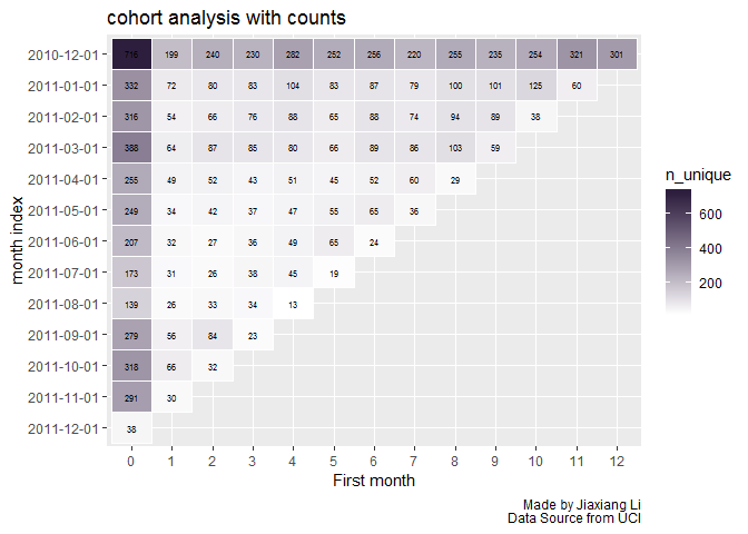
cohort_ana %>% 
    ggplot(aes(y = first_invoice_month %>% 
                   as.factor() %>% 
                   fct_reorder(first_invoice_month,.desc = T)
               ,x = str_sub(cohort_index_month,1,7) %>% 
                   fct_reorder(cohort_index_month)
               )) +
    geom_tile(aes(fill = n_unique),color='white') +
    # color 是加边框
    geom_text(aes(label = n_unique),size = 2) +
    scale_fill_gradient(low = 'white', high = '#2d1e3e', space = 'Lab', na.value = 'white') +
    # 改变瓦砾的颜色
    labs(
        x = 'First month'
        ,y = 'month index'
        ,title = 'cohort analysis with counts'
        ,caption = 'Made by Jiaxiang Li\nData Source from UCI'
    )

cohort_ana %>% 
    ggplot(aes(y = first_invoice_month %>% 
                   as.factor() %>% 
                   fct_reorder(first_invoice_month,.desc = T)
               ,x = str_sub(cohort_index_month,1,7) %>% 
                   fct_reorder(cohort_index_month)
               )) +
    geom_tile(aes(fill = avg_quantity),color='white') +
    # color 是加边框
    geom_text(aes(label = avg_quantity),size = 2) +
    scale_fill_gradient(low = 'white', high = '#2d1e3e', space = 'Lab', na.value = 'white') +
    # 改变瓦砾的颜色
    labs(
        x = 'First month'
        ,y = 'month index'
        ,title = 'cohort analysis with average quantity'
        ,caption = 'Made by Jiaxiang Li\nData Source from UCI'
    )

Urbonas, Karolis. 2018. “Customer Segmentation in Python.” 2018. <https://www.datacamp.com/courses/customer-segmentation-in-python>.