使用 RMarkdown 的 child 参数，进行文档拼接。
这样拼接以后的笔记方便复习。
相关问题提交到 Issue

1 直观理解 Interpretation

The first principal component direction of the data is that along which the observations vary the most. (James et al. 2013, 231)

There is also another interpretation for PCA: the first principal component vector defines the line that is as close as possible to the data. (James et al. 2013, 231)

PC1表示的是样本波动最多的方向。
PC1表示的是一个向量，最贴近数据。

2 合成指数

2.1 工业界应用

PCA可以用来做 data driven 的指数，比如使用第一个PC作为指数(Peña, Smucler, and Yohai 2020,Figure 3)，并且可视化上，可以通过corplot函数，看变量相关性集中的地方，可以看出权重大的变量。 (Pflieger 2018, 1–2)

Because components are determined based on the correlations PCA uses the correlations to determine the components that cover as much as possible of the original variance.

因为PCA是基于变量间的相关性来做PC的。(Pflieger 2018, 4)

$\text{PC}_i$是描述方差top i的向量，满足以下公式，因此是方差累计的排序。因此需要标准化(Pflieger 2018, 6; 陈强 2018)。

\[\sum\text{Var}(X_i) = \sum\text{Var}(\text{PC}_i)\]

\[\text{component importance} = \frac{\text{PC}_i}{\sum\text{Var}(\text{PC}_i)} = \frac{\text{PC}_i}{\sum\text{Var}(X_i)} = \frac{\text{PC}_i}{\sum i}\]

标准化后，看重要性就直接除以变量数量。因此这也引申出Kaiser-Guttman Criterion，Eigenvalue > 1，也就是一个$\text{PC}_i$的方差必须大于一个原始$X_i$的方差，否则就没有降维的意义。

通过看$X_i \sim \text{PC}_i$ 关联表，定义$\text{PC}_i$为指数，如 low return，low activity 等等。并且可以看到$X_i \sim \text{PC}_i$的对应loading，这个是两者的相关性，通过prcomp(...)$rotation函数实现。并且利用关联表可以计算每个id的在每个指数下的得分。(Pflieger 2018, 5)

PCA comp 的决定，有三种方法(Pflieger 2018, 10)，

screeplot()函数实现，就是看图
Kaiser-Guttmann criterion，就是看$\text{Var}(\text{PC}_i) > 1$，因此也可以看是否显著大于1(Wikipedia contributors 2018a; Larsen and Warne 2010; Warne and Larsen 2014)。
或者看累计解释方差的70%

2.2 学界应用

image

处理方法为

先PCA得到每个变量和 PCs 的 loading
取行最大 rowMax，每个 PC 中的 loading 只保留行最大的，其他设为0

Three principal components extract most of the variance from the original dataset. Control corruption (0.90), rule of law (0.91), voice (0.83), effectiveness (0.90), political stability (0.60) and security and regulatory quality (0.86) have the highest factor loading on the first compo nent. This component is labeled “governance quality index” (GOVI). This GOVI dimension explains most of the variance from the dataset: 46.69% (Capelle-Blancard et al. 2019)

Specifically, the first component, which represents the first composite index: “governance quality index” (GOVI) is computed as follows: GOVI = 0.19xcorruption + 0.20xrule + 0.16xvoice + 0.19xeffectiveness + 0.08xstability + 0.18xregulatory. (Capelle-Blancard et al. 2019)
处理后，对 PCs 再进行标准化。因为主成分非常强调标准化，因为它是解释方差的算法，不然方差大的变量会表现高估。

normalized sum of squared loading(Capelle-Blancard et al. 2019)
```
library(magrittr)
```
```
## Warning: package 'magrittr' was built under R version 3.6.1
```
```
c(.9,.91,.83,.9,.6,.86) %>% 
    magrittr::raise_to_power(2) %>% 
    {./sum(.)}
```
```
## [1] 0.1911910 0.1954633 0.1626068 0.1911910 0.0849738 0.1745740
```
取平方和做分母。
最后对PCs对方差的解释占比作为PCs的权重，构建 ESGGI

For example, the weighting of the first intermediate composite index is 0.45 (45%), calculated as follows: 5.65/(5.65 + 3.52 + 3.27)(Capelle-Blancard et al. 2019)
ESGGI = 0.45xGOVI + 0.30xSODI + 0.25xENVI (Capelle-Blancard et al.

这种处理方法可以这么认为。

首先不是所有权重都使用，类似于 OLS 和 Lasso 的区别，把小的权重设为0，做了正则化的处理，保证指数更泛化。
其次最后取平方和做分母，相当于做标准化。

补充，

是的，你可以看下这样处理后是不是新的loadings 平方和后等于1？是不是就是一个长度为1的单位向量了。

The third step involves the rotation of factors. Rotation is a standard step in factor analysis. It provides a criterion for eliminating the indeterminacy implicit in factor analysis results. (Capelle-Blancard et al. 2019)

这个处理叫做 factor rotations。目的是把一个 PCs 内较弱的(比如绝对值较小)的变量删除。

The rotation changes the factor loadings and consequently the interpretation of the factors, but the different factor analytical solutions are mathematically equivalent in that they explain the same portion of the sample variance.

当然这样的处理肯定是会改变主成分的解读。

var_name	PC1_unrotated	PC2_unrotated	PC3_unrotated	PC1_rotated	PC2_rotated	PC3_rotated
X_ 7	0.5281055	0.2460877	0.5440660	0.0000000	0.0000000	0.5440660
X_ 4	0.8830174	0.5726334	0.9942698	0.0000000	0.0000000	0.9942698
X_ 3	0.4089769	0.6775706	0.6405068	0.0000000	0.6775706	0.0000000
X_ 6	0.0455565	0.8998250	0.7085305	0.0000000	0.8998250	0.0000000
X_ 10	0.4566147	0.9545036	0.1471136	0.0000000	0.9545036	0.0000000
X_ 1	0.2875775	0.9568333	0.8895393	0.0000000	0.9568333	0.0000000
X_ 9	0.5514350	0.3279207	0.2891597	0.5514350	0.0000000	0.0000000
X_ 2	0.7883051	0.4533342	0.6928034	0.7883051	0.0000000	0.0000000
X_ 8	0.8924190	0.0420595	0.5941420	0.8924190	0.0000000	0.0000000
X_ 5	0.9404673	0.1029247	0.6557058	0.9404673	0.0000000	0.0000000

Factor rotation is obtained using the varimax method, which attempts to minimize the number of variables that have high loadings (so-called salient loadings) on the same factor. (Capelle-Blancard et al. 2019)

以上就是 varimax 处理方式，通过处理后，我们发现系数较小的变量在 PCs 进行了移除，达到了 vari(able) - max 的目的，只保留最高的 loadings。

This is a transformation of factorial axes that makes it possible to approximate a “simple structure” of the factors, in which each indicator is “loaded” exclusively on one of the retained factors. This enhances the interpretability of these factors. (Capelle-Blancard et al. 2019)

当然类似于 Lasso，我们让每个 PCs 拥有更少的变量，实现简单结构，同时也让每个变量只出现在某个 PCs，更加体现了 PCA 的“正交化”，增加 PCs 的可解释性。不会出现一个变量决定多个变量，这样难以解释。

3 practice

3.1 做分类

参考文档。

spam <- read_csv('https://raw.githubusercontent.com/JiaxiangBU/picbackup/master/spam.csv')
spam_edited <- 
spam %>% 
    na.omit() # 自己处理下缺失值
pca_model <- 
    prcomp(spam_edited %>% select(-type),
           center = TRUE,scale. = TRUE)
eda_data <- 
predict(pca_model) %>% 
    as_tibble() %>% 
    select(1:2) %>% 
    bind_cols(spam_edited %>% select(type))
eda_data %>% 
    mutate(type = as.factor(type)) %>% 
    ggplot(aes(x = PC1, y = PC2, col = type)) + 
        geom_point()

3.2 PCA in Python

代码主要参考 Pedregosa et al. (2011) 的开发手册。

import pandas as pd
data = pd.read_csv("../tutoring/dataMat.csv")

# data.columns.values
data = data[['fst_add_gamble_app_cnt_r15d','fst_add_app_cnt_r30d', 'fst_add_p2p_app_cnt_r30d']]

from sklearn.decomposition import PCA
pca = PCA(n_components=2)
pca.fit(data.values)
pca_output = pca.transform(data.values)
print pca.explained_variance_ratio_
print pca.singular_values_
print pca.components_
# print pca_output

4 weakness

最后发现用$\text{PC}_i$去做回归虽然避免了过拟合，但是$\text{adj.R}^2$下降的快。实验证明，21个$X_i$比20个$\text{PC}_i$好。(Pflieger 2018, 15)

但是提供一个系统性的解决方案，使用PCR(Wikipedia contributors 2018b)+Lasso。

5 methodology (陈强 2018)

假设有$p$维向量

\[x = [x_1,\cdots,x_p]'\]

根据线性代数，构建

\[\text{PC}_1 = c_1 x_1 + \cdots + c_p x_p\]

使其信息量最大，假设信息量最大，就是这个构建出来的向量的方差最大¹。因此不断调节向量$[c_1,\cdots,c_p]$使$\text{Var}(\text{PC}_1|c_1,\dots,c_p)$最大。因此空间几何上，在一个$p$维空间，不断旋转一个向量，找到匹配的权重$[c_1,\cdots,c_p]$，使得$\text{Var}(\text{PC}_1|c_1,\dots,c_p)$最大。

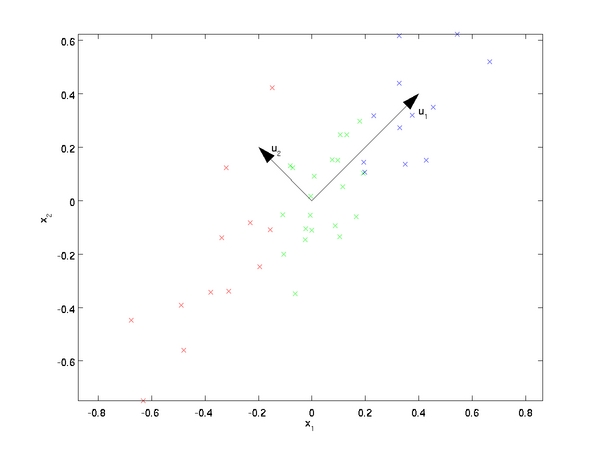
如图二维空间上，旋转到$\text{PC}_1$最大的方向了

然后在正交方向上，第二个为$\text{PC}_2$，一次类推。

我们得到

\[\begin{alignat}{2} z_1 = \alpha_1'\mathrm{x} \\ \vdots \\ z_p = \alpha_p'\mathrm{x} \\ \end{alignat}\]

由上可知，

\[z_i \perp z_j | i \neq j\] \[\alpha_i \perp \alpha_j | i \neq j\]²

因此，

\[\max_{\alpha} \mathrm{Var (\alpha' x)} = \mathrm{\alpha'}\Sigma \mathrm{\alpha'} \\ \mathrm{s.t. \alpha' \alpha = 1} \]

这里的 $\mathrm{\alpha} = [\alpha_1,\cdots,\alpha_p]$

$\Sigma$是$\mathrm{x}$的协方差矩阵，特征根为$\lambda = [\lambda_1,\cdots,\lambda_p]$。通过拉格朗日乘数法、一阶求导求得。由于$z_i \perp z_j | i \neq j$，因此$\Sigma$的特征根就是$\mathrm{Var(z_i)}$

6 debugging

当$x_1,\dots,x_n$存在是常数或者空时，会出bug(Rothwell 2016)。

一般的办法是

select_if(~sum(is.na(.))!=0)
select_if(~var(.))!=0)

7 more reading

应用,中文: http://www.cnblogs.com/pinard/p/6243025.html
pca.components_: https://stackoverflow.com/questions/23294616/how-to-use-scikit-learn-pca-for-features-reduction-and-know-which-features-are-d
components_ : array, shape (n_components, n_features)
1. Principal axes in feature space, representing the directions of maximum variance in the data. The components are sorted by explained_variance_. 参考: http://scikit-learn.org/stable/modules/generated/sklearn.decomposition.PCA.html

8 非线性表达

library(tidyverse)

https://blog.umetrics.com/what-is-principal-component-analysis-pca-and-how-it-is-used

PCA 效果展示，选图片。

library(imager)

# load the image and look at the image properties
image = load.image(here::here("figure/base-image.png"))
image

## Image. Width: 1025 pix Height: 647 pix Depth: 1 Colour channels: 3

# convert image data to data frame
image_df = as.data.frame(image)
image_df %>% 
    summarise(n_distinct(x,y))

1025 * 647

## [1] 663175

head(image_df) # 灰度的

image_mat = matrix(image_df$value,
                   nrow = 647,
                   ncol = 1025,
                   byrow = TRUE)

# visualize the image
image(t(apply(image_mat, 2, rev)), col = grey(seq(0, 1, length = 256)))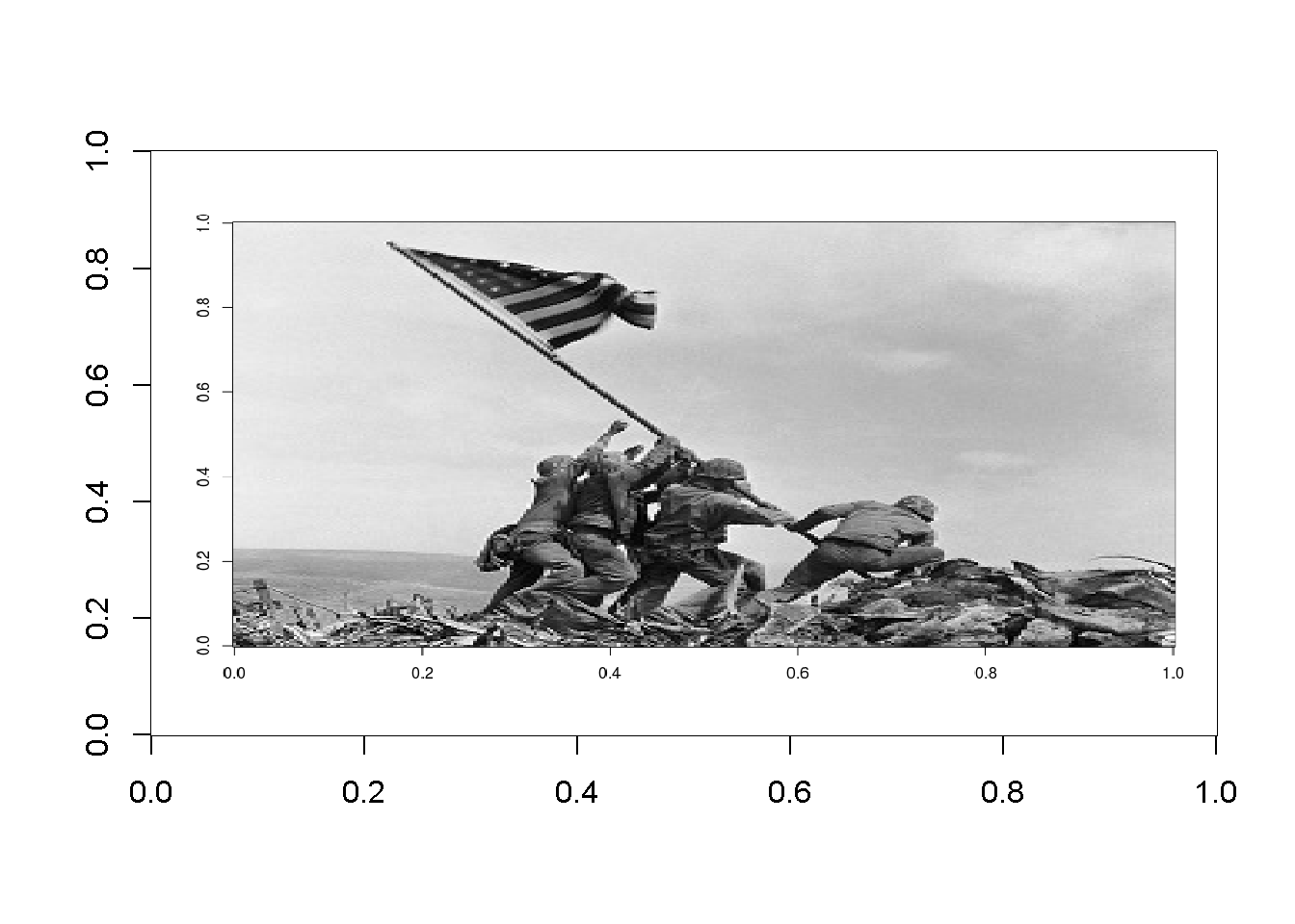

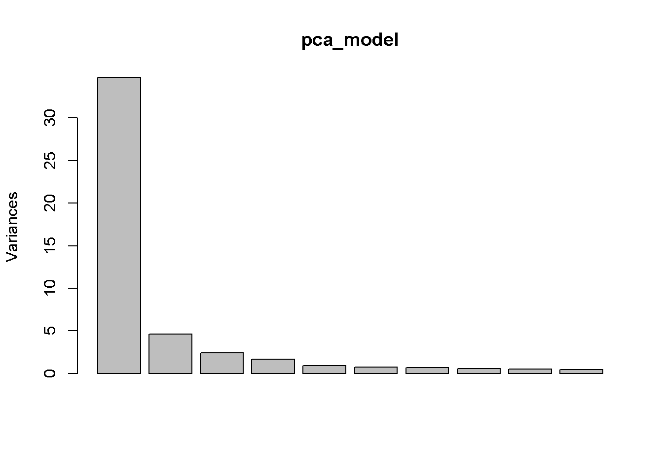
# pca analysis
pca_model = prcomp(image_mat)

# plot the scree plot
plot(pca_model)

很明显，PC1已经拿到40%的权重了。

# Reconsturction and plotting
par(mfrow= c(3,3))
recon_fun = function(comp){
  recon = pca_model$x[, 1:comp] %*% t(pca_model$rotation[, 1:comp])
  image(t(apply(recon, 2, rev)), col=grey(seq(0,1,length=256)), main = paste0("Principle Components = ", comp))
}

# run reconstruction for 1:17 alternating components
lapply(seq(1,18, by = 2), recon_fun)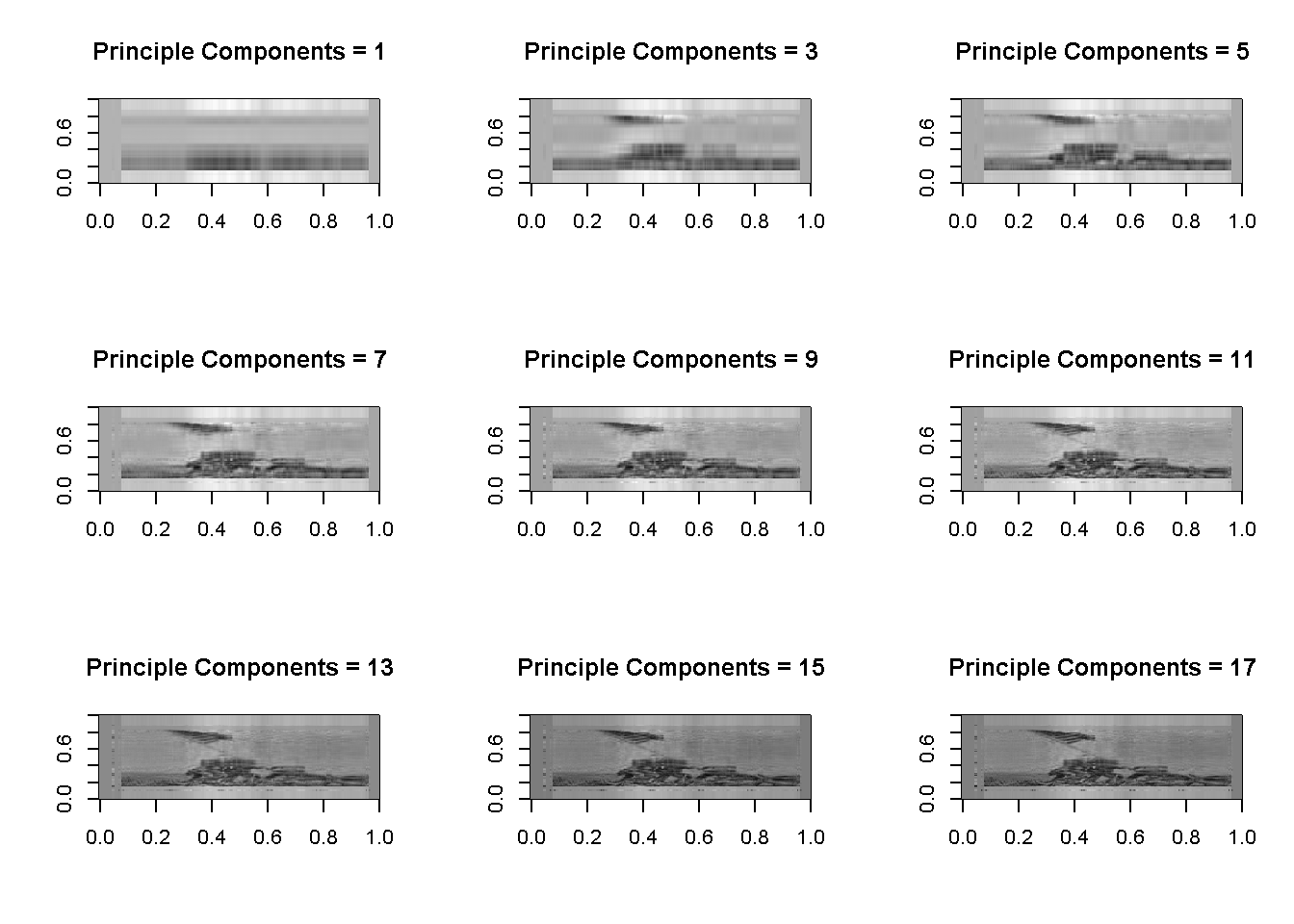

## [[1]]
## NULL
## 
## [[2]]
## NULL
## 
## [[3]]
## NULL
## 
## [[4]]
## NULL
## 
## [[5]]
## NULL
## 
## [[6]]
## NULL
## 
## [[7]]
## NULL
## 
## [[8]]
## NULL
## 
## [[9]]
## NULL

# 从1到11后才能表现好一些。

显然 PCA 的效果并不好，还是要多考虑非线性关系。

附录

参考文献

Capelle-Blancard, Gunther, Patricia Crifo, Marc-Arthur Diaye, Rim Oueghlissi, and Bert Scholtens. 2019. “Sovereign Bond Yield Spreads and Sustainability: An Empirical Analysis of Oecd Countries.” Journal of Banking & Finance 98: 156–69. https://doi.org/https://doi.org/10.1016/j.jbankfin.2018.11.011.

James, Gareth, Daniela Witten, Trevor Hastie, and Robert Tibshirani. 2013. An Introduction to Statistical Learning with Applications in R. 8th ed. Springer New York.

Larsen, Ross, and Russell T. Warne. 2010. “Estimating Confidence Intervals for Eigenvalues in Exploratory Factor Analysis.” Behavior Research Methods 42 (3): 871–76. https://doi.org/10.3758/BRM.42.3.871.

Pedregosa, F., G. Varoquaux, A. Gramfort, V. Michel, B. Thirion, O. Grisel, M. Blondel, et al. 2011. “Scikit-Learn: Machine Learning in Python.” Journal of Machine Learning Research 12: 2825–30.

Peña, Daniel, Ezequiel Smucler, and Victor J. Yohai. 2020. “gdpc: An R Package for Generalized Dynamic Principal Components.” Journal of Statistical Software, Code Snippets 92 (2): 1–23. https://doi.org/10.18637/jss.v092.c02.

Pflieger, Verena. 2018. “Marketing Analytics in R: Statistical Modeling: Reducing Dimensionality with Principal Component Analysis.” DataCamp. 2018. https://www.datacamp.com/courses/marketing-analytics-in-r-statistical-modeling.

Rothwell, Joseph. 2016. “How to Solve Prcomp.default(): Cannot Rescale a Constant/Zero Column to Unit Variance.” 2016. https://stackoverflow.com/questions/40315227/how-to-solve-prcomp-default-cannot-rescale-a-constant-zero-column-to-unit-var.

Warne, Russell T, and Ross Larsen. 2014. “Evaluating a Proposed Modification of the Guttman Rule for Determining the Number of Factors in an Exploratory Factor Analysis.” Psychological Test & Assessment Modeling 56 (1): 104–23.

Wikipedia contributors. 2018a. “Factor Analysis — Wikipedia, the Free Encyclopedia.” https://en.wikipedia.org/w/index.php?title=Factor_analysis&amp;amp;amp;amp;amp;amp;oldid=853104366.

———. 2018b. “Principal Component Regression — Wikipedia, the Free Encyclopedia.” https://en.wikipedia.org/w/index.php?title=Principal_component_regression&oldid=835543805.

刘建平. 2016. “主成分分析（PCA）原理总结.” 2016. http://www.cnblogs.com/pinard/p/6239403.html.

陈强. 2018. “为何你还没理解主成分分析.” 2018. https://mp.weixin.qq.com/s/_2SirRp3DGbbLHHHV4xqoA.

感觉PCA 剔除的也不是噪音，而是某方向上方差很小的，也就是这个方向是常数，信息值很低而已。然而噪音并不是常数，而是方差很大的。同时剔除的常数，也很可能是含有重要的信息，一些规则 (刘建平 2016)。

刘建平 (2016) 认为comp1选择 $\mu_1$的原因是，
- 因为各个点离这个超平面或者直线最近，可以用这个直线来代表更多信息。
- 点在这条线上的投影，比较分散，也就是方差大，信息充分。
↩︎
看图，还真是正交的。↩︎

主成分分析学习笔记

主成分分析学习笔记

1 直观理解 Interpretation

2 合成指数

2.1 工业界应用

2.2 学界应用

3 practice

3.1 做分类

3.2 PCA in Python

4 weakness

5 methodology (陈强 2018)

6 debugging

7 more reading

8 非线性表达

附录

参考文献

主成分分析 学习笔记

1 直观理解 Interpretation

2 合成指数

2.1 工业界应用

2.2 学界应用

3 practice

3.1 做分类

3.2 PCA in Python

4 weakness

5 methodology (陈强 2018)

6 debugging

7 more reading

8 非线性表达

附录

参考文献

主成分分析学习笔记