Hive/Impala 学习笔记
2020-08-02
If you look at Oracle’s official documentation on SQL, it says it’s still pronounced “sequel” [2]. However, if you look at MySQL’s official documentation, it says “MySQL” is officially pronounced “‘My Ess Que Ell’ (not ‘my sequel’)” [3], and Wikipedia says SQL is officially pronounced “S-Q-L” and references an O’Reilly book on the subject [4]. So this is no help, the major sources aren’t agreeing on the way it’s “officially” pronounced. (Gillespie 2012) Since the language was originally named SEQUEL, many people continued to pronounce the name that way after it was shortened to SQL. Both pronunciations are widely used and recognized. As to which is more “official”, I guess the authority would be the ISO Standard, which is spelled (and presumably pronounced) S-Q-L. (Gillespie 2012)
Don Chamberlin 在邮件里面回复,这门语言一开始读 sequel,后来慢慢简短,读 S-Q-L。 所以单独读 SQL 发音 [ˈsikwəl],读 MySQL,读成 My-S-Q-L。
1 建表逻辑 create tbl
1.1 impala 数据清理的流程
建表流程
- ID 表
create table,因为ID表需要反复用,因此不需要重复跑code- 建立新表,最好加上注释,流程参考 1.2
- 中间表
with,因为中间表的逻辑可能只用少数几次,因此不需要建立一个表,占用资源
中间表适用方式
create table a
create table b
create table c
create table d

select *
from a
join b
join c
join d
ID 表适用方式
with a as ()
, b as ()
, c as ()
, d as ()

select *
from a
join b
join c
join d
X表跑全量的原因是
- 某个X表,全量样本是100,
- 分表逻辑参考 1.3
- ID表,样本是10
create table x1 as ()
size = 100

create table id as ()
size = 10

from id
size = 10
left join x1
size = 100- 形成全量表
size = 10 - 如果ID进行更换,那么X表不需要修改,只需要修改ID表,进行
join即可。- 而且一般来说ID表是少量的,X部分表是多量的,这也满足节约资源的思路,见 2.4
形成宽表的检查
- 最后查看是否样本因为
left join增加(重复样本问题),并且 - 有没有空值(没有匹配上是正常吗?)
1.2 Impala/Hive 建表加注释的方式
- 创建好临时表,标注主要变量(1%,50%,99%的位置的注释),其他的参考 人工智能爱好者社区 (2018) 这篇文章code的写法。
- 建立好生成表的注释,下方会解释
describe formatted下注释是否都标注完成
假设中间表逻辑为
建立好生成表的注释
create table xxx.test_add_sth
(
    x1 int comment '注释: 这是一个连续变量'
    ,x2 string comment '注释: 这是一个文本变量'
)
comment '注释: 表的说明和注意事项'
将临时表插入生成表中
Table Parameters:   NULL                    NULL
                    comment                 注释: 表的说明和注意事项
                    transient_lastDdlTime   1535523988
最后发现检查下表的注释是否都标注完成。
1.3 特征变量分表采集
表分三类
- ID表
- y表
- 若干的x表
分开建立中间表,主要理由如下
- 如果y表修改了,可以避免跑全表(主要是x),因为一般x表有文本处理,很慢。
- ID表为了样本很干净,会进行很多处理,在处理同时,可以使得y表和x表不受到影响
- debug 找错时,可以独立进行
- 使得代码模块化,readable 易于翻译 和 别人QA
模型数据中的特征变量\(x\)按照功能切分分表记录,因为
- 宽表执行速度慢
- 一个字段的修改,如果重刷一个宽表,修改速度太慢,因为一般一个x表要求是全量,那么在一张宽表里,会发生
- 全量样本大,执行慢
- 嵌套join,容易出错,参考 2.1
- 因此按照功能区分,当一个功能的表需要修改逻辑时,不需要跑其他表
1.4 drop/create table 和 exists
主要参考 Capriolo, Wampler, and Rutherglen (2012) 的书。
1.5 批量删除表 in R
sqlDrop("xxx.vars_name")加一个for loop 就可以批量删除了。
for (i in 1:100){
  sqlDrop(paste("xxx.vars_name",i,sep="_"))
}这里可以把所有xxx.vars_name_*的表删除。
1.6 show stats (Cloudera, Inc. 2018b)
compute stats可以使得表的join等指令运行加快,以下代码可以检验是否compute stats。
show column stats看表内每个字段n_distinct、n_nulls、max_size和avg_size。show table stats- 通常出现的
-1表示空的意思。
1.7 建表不要以数字开头
否则无法INVALIDATE METADATA等命令
1.8 invalidate metadata
invalidate metadata + table name,相当把Hive的表放到impala中。
但是Hive 可以直接调用impala的数据。
(Capriolo, Wampler, and Rutherglen 2012)
1.9 alter table and parts (Cloudera, Inc. 2018a)
alter table xxx.learn_add_comment rename to  xxx.learn_add_comment2;
alter table xxx.learn_add_comment2 change x2  x3 string;
alter table xxx.learn_add_comment2 change x3 x4 string comment 'x4';rename: 方便大家统一命名表,而不需要重新跑表change: 方便大家修改变量,而不需要重新跑表
参考 w3cschool
参考 w3xue
1.10 insert table
insert overwrite table: delete and update …insert into table: update,more here
活用alter和insert,这样不至于重复delete和create表格,浪费时间。
1.11 报表命名 (Cloudera, Inc. 2018c)
select name as "leaf node" from tree one
+--------------+
| leaf node    |
+--------------+
| bats         |
| lions        |
| tigers       |
| red kangaroo |
| wallabies    |
+--------------+这样就可以展示性报表,如变量leaf node
1.12 impala中文命名
select 1 as 变量
1.13 快速sim表 (Cloudera, Inc. 2018c)
2 并表 join
2.1 多层嵌套
WITH JOBS (id, SurName, JobTitle) AS
(
    SELECT ID, Name, Position
    FROM employee
    WHERE Position like '%Manager%'
),
SALARIES (ID, Salary) AS
(
    SELECT ID, Salary
    FROM ITSalary
    WHERE Salary > 10000
)
SELECT JOBS.NAME, JOBS.POSITION, JOBS.Salary
FROM JOBS
INNER JOIN SALARIES
on JOBS.ID = SALARIES.ID;o
在 WITH 表头标记变量名称,方便用户了解表结构。不然用户需要查询 WITH 内 select 中每个变量,如果变量是在 transformation 中,需要看 ... as x1 这样很麻烦。
(Egarter 2019)
2.2 semi/anti join
依然可以使用[shuffle]加快运行速度。
主要参考 Capriolo, Wampler, and Rutherglen (2012) 的书。
select a.userid from
(select * from xxxlistingautoflowsysprocess limit 10) a
left semi join [shuffle]
(select * from xxxlistingautoflowsysprocess limit 5) b
on a.userid = b.userid
semi join anti join,这个可以实现差集等操作。
- The UNION [ALL], INTERSECT, MINUS Operators impala、Hive 中没有
- What are the biggest feature gaps between HiveQL and SQL? - Quora No regular UNION, INTERSECT, or MINUS operators.
LEFT SEMI JOIN=whereon conditionin ()(Edward, Dean, and Jason 2012)
2.2.1 semi join 替换 (subquery) (Cloudera, Inc. 2018c)
select name as "leaf node" from tree one
where not exists (select parent from tree two where one.id = two.parent);
2.2.2 outer join, inner join, semi join 区别
with tbl_1 as (
    select 1 as x1 union all
    select 2 as x1 union all
    select 3 as x1 union all
    select 4 as x1 union all
    select 5 as x1 union all
    select 6 as x1
)
select *
from tbl_1 b
-- inner join [shuffle] (
left semi join [shuffle] (
    select 1 as x2 union all
    select 2 as x2 union all
    select 3 as x2 union all
    select 4 as x2 union all
    select 5 as x2 union all
    select 6 as x2
) a
on b.x1 < a.x2
-- 6 * 6 lines
2.2.3 mysql中的实现
where (not) in (on ...)就是semi/anti joininner join on !=就是anti join。但是要保重主表是唯一的Key
2.2.4 mysql where 进行 left semi join
2.3 union all和union
The
UNIONkeyword by itself is the same asUNION DISTINCT. Because eliminating duplicates can be a memory-intensive process for a large result set, preferUNION ALLwhere practical. (That is, when you know the different queries in the union will not produce any duplicates, or where the duplicate values are acceptable.) (I. Cloudera 2015; Cloudera, Inc. 2018d)
2.4 from small join large
Hive also assumes that the last table in the query is the largest. (Edward, Dean, and Jason 2012)
因此用小表去JOIN大表。
2.5 sql里的bind_cols
with tbl_1 as
(
  select null as x1, 1 as id union all
  select 1 as x1, 2 as id  union all
  select 2 as x1, 3 as id  union all
  select 3 as x1, 4 as id
)
select a.x1,b.x2,c.x3
from tbl_1 a
left join [shuffle]
(
  select null as x2, 1 as id  union all
  select 1 as x2, 2 as id  union all
  select 2 as x2, 3 as id  union all
  select 3 as x2, 4 as id
) b
on a.id = b.id
left join [shuffle]
(
select null as x3, 1 as id  union all
select 1 as x3, 2 as id  union all
select 2 as x3, 3 as id  union all
select 3 as x3, 4 as id
) c
on a.id = c.id
2.6 impala JOIN 表出问题debugging方法
例如,样本变少
- 检验主表
- 主表没有问题,检验on条件
- ON条件没有问题,检验副表
3 运算符 operators
3.1 运算符 arithmetic operators
3.1.1 A <=> B
甚至,A is null and B is null \(\to\) A <=> B 成立。
(Bansal, Chauhan, and Mehrotra 2016, 137)
因此可以转换为
(A is null and B is null) or A=B。
注意这里不能等价于(A is null and A=B) or A=B。
因为null = null即使为真,也是null,因为null不能用等价符号识别,见3.1.6。
with table_1 as
(
  select NULL as x1, NULL as x2
  union all
  select 1 as x1, 1 as x2
  union all
  select NULL as x1, 1 as x2
  union all
  select 1 as x1, NULL as x2
)
select *, x1 <=> x2 as result
from table_1这样会产生\(3 \times 3\)的数据。
with tbl_1 as (
    select null as x1 union all
    select null as x1 union all
    select null as x1
)
select a.x1,b.x1
from tbl_1 a
inner join [shuffle] (
    select null as x1 union all
    select null as x1 union all
    select null as x1
) b
on a.x1<=>b.x1因此空值也是一个level的话,去join,可以使用<=>
3.1.2 IS DISTINCT FROM Operator (Cloudera, Inc. 2018e)
SELECT
1 is distinct from NULL
,1 != NULL
,null is not distinct from null
,null != null
,null <=> null
,null != null or (null is null and null is null)
is distinct from近似于!=is not distinct from近似于=
但是前者更考虑null的情况。
因此
is not distinct from = <=> = A = B OR (A IS NULL AND B IS NULL)
3.1.3 bitwise 暂时用不到
A & BXORA ^ B~A
3.1.4 Range Access Method for Multiple-Part Indexes
with a as (
select 0.01313 as pred2
)
select
case
    when 9.45e-05 < pred2 <=  0.00154 then 1
    when     0.13 < pred2 <=    0.431 then 1
    when   0.0134 < pred2 <=     0.13 then 2
    when  0.00154 < pred2 <=   0.0134 then 3
    when    0.994 < pred2 <=        1 then 4
    when 2.22e-16 < pred2 <= 9.45e-05 then 5
    when    0.431 < pred2 <=    0.775 then 6
    when    0.775 < pred2 <=    0.994 then 6
end as pred
from a- 多个等号连接是可以直接使用的(Oracle Corporation and/or its affiliates 2018d)。
9.45e-05是符合科学计数法可以直接使用(Oracle Corporation and/or its affiliates 2018b)。-infmysql不能支持 (Oracle Corporation and/or its affiliates 2018d)
3.1.5 between函数
with tbl_1 as
(
SELECT '2018-01-01' as x1 union all
SELECT '2018-01-02' as x1 union all
SELECT '2018-01-10' as x1
)
select x1
from tbl_1
where x1 between '2018-01-01' and '2018-01-10'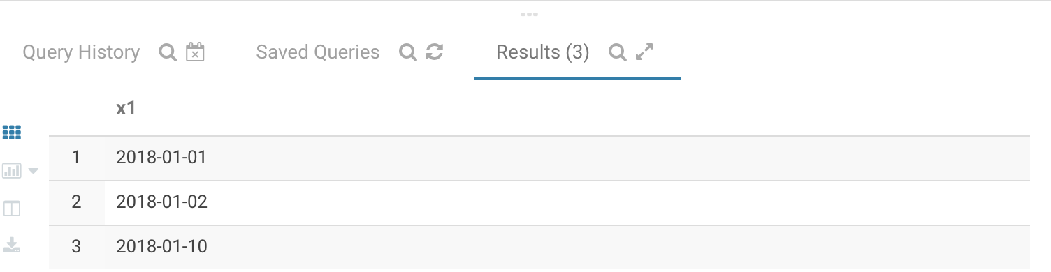
都是闭区间。
3.1.6 A NOT IN (NULL)
A NOT IN (value1, value2, …)It will return TRUE if the value of A is not equal to any of the given values. [pp.143]
equal 相等的算法,NULL值是不能够使用的。
select NULL = NULL, NULL != NULL, NULL is not null, NULL is NULL
NULL, NULL, false, true因此,A NOT IN (NULL) 相当于判断 A != NULL,那么反馈都是NULL,如果写入where条件中,反馈就是0行。
3.2 logical operators
with table_1 as
(
  select NULL as x1
  union
  select 1 as x1
  union
  select 2 as x1
  union
  select 3 as x1
  union
  select 4 as x1
  union
  select 5 as x1
)
select x1
from table_1
-- where x1 > 2 && x1 < 4
where !(x1 > 2 && x1 < 4) || (x1 > 2 && x1 < 4) is null&&=and||=or
否命题:
NOT和!是不完备的还需要() is null。
(Bansal, Chauhan, and Mehrotra 2016, 148)
3.3 is_inf和is_nan
Infinity and NaN can be specified in text data files as inf and nan respectively, and Impala interprets them as these special values. They can also be produced by certain arithmetic expressions; for example,
1/0returnsInfinityandpow(-1, 0.5)returnsNaN.Or you can cast the literal values, such asCAST('nan' AS DOUBLE)orCAST('inf' AS DOUBLE). (Cloudera 2018b)
is_inf(double a): Tests whether a value is equal to the special value “inf”, signifying infinity.is_nan(double a): Tests whether a value is equal to the special value “NaN”, signifying “not a number”.
4 函数 function
4.1 函数查询
这里直接搜索,非常方便,不需要记忆函数的名称。
4.2 built-in function
很多不知道应用场景 (Capriolo, Wampler, and Rutherglen 2012, 83–84)
round()round(d,N)floor(d)反馈最大整数,如果要反馈最大十位数,先除以10再乘以10ceil(d)反馈最小整数,如果要反馈最大十位数,先除以10再乘以10rand(seed),反馈的是integer
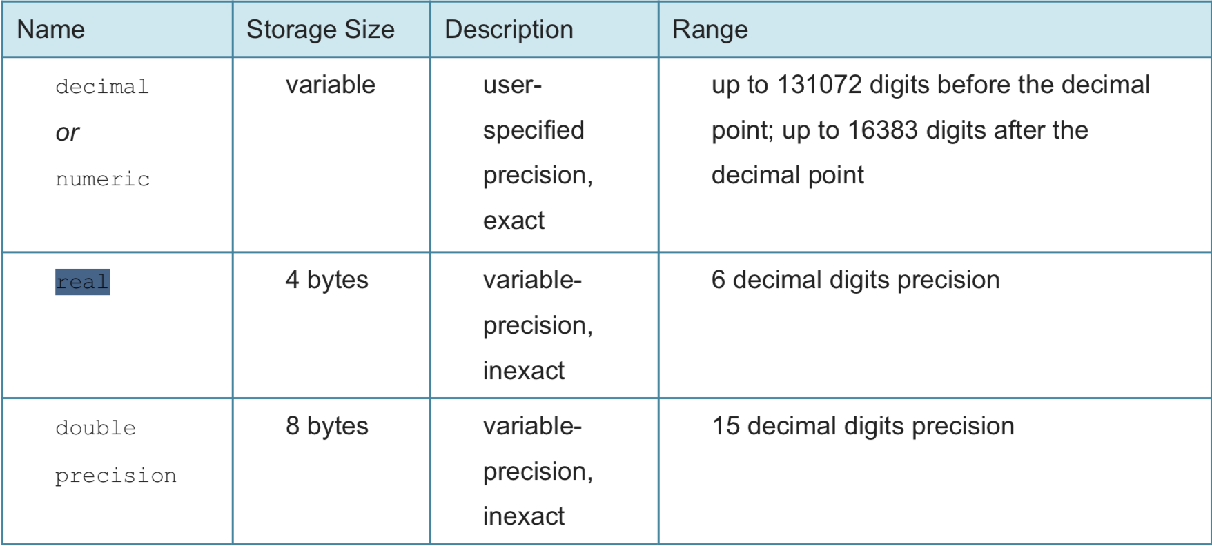
4.2.1 decimal可以不受到float假设影响
select cast(0.xxx as decimal(20,1))4.2.2 time 函数
4.2.2.1 把秒、分秒位清洗
from_timestamp(datetime timestamp, pattern string)函数很好。
参考: cloudera,(I. Cloudera 2015)
自定义时间。
把一个时间变量,转换为string。
所以最后还是需要cast(... as timestamp)
配合to_timestamp,可以把秒、分秒位清洗了。
4.2.2.2 from_unixtime
from_unixtime(bigint unixtime[, string format])输入为INT,输出为string。
select from_unixtime(1392394861,"yyyy-MM-dd HH:mm:ss.SSSS");
select from_unixtime(1392394861,"yyyy-MM-dd");


select from_unixtime(to_unix_timestamp('16/Mar/2017:12:25:01 +0800', 'dd/MMM/yyy:HH:mm:ss Z')), 'easy way' as type
-- 替换成统一格式,然后再转换
参考 博客园
4.2.2.3 add_?*
替代为
+或者-的interval N days/months ...
4.2.2.4 extract
SELECT date_part("year","2017-01-01 11:00:00")
SELECT date_part("month","2017-01-01 11:00:00")
SELECT date_part("day","2017-01-01 11:00:00")
SELECT date_part("hour","2017-01-01 11:00:00")
SELECT date_part("second","2017-01-01 11:00:00")
替代为
days, months
4.2.2.5 cast(... as timestamp) 时间不会变
select due_date, cast(due_date as timestamp) as due_date_checked
from xxxtb_loan_debt
4.2.2.6 求时间变量的月底变量
adddate(
    cast(
        concat(
            substr(
                cast(
                add_months(t,1)
                as string
                ),1,7),
            "-",
            "01"
            )
        as TIMESTAMP
        ),-1
    )
as end_of_month
求时间变量的月底时间。
t先加一个月,add_months(t,1)
cast(
  add_months(t,1)
  as string
  ),1,7)
提取年份和月份。
substr假设日为1
最后cast为TIMESTAMP
adddate倒数一天,因此就是本月的最后一天了。
4.2.2.7 日期差
datediff(timestamp enddate, timestamp startdate)(mysql也可以用)(Cloudera 2018a)
4.2.2.8 where 条件中时间比较时,string格式默认转为时间格式
with tbl_2 as
(
    with tbl_1 as
    (
      select '2018-01-01 08:00:00' as tm union all
      select '2018-01-02 08:00:00' as tm union all
      select '2018-01-01 09:00:00' as tm union all
      select '2018-01-03 08:00:00' as tm union all
      select '2018-01-01 10:00:00' as tm union all
      select '2018-01-04 08:00:00' as tm union all
      select '2018-01-01 13:00:00' as tm union all
      select NULL as tm
    )
    select cast(tm as timestamp) as tm
    from tbl_1
)
select tm
from tbl_2
where tm > '2018-01-02'
因此这里的'2018-01-02'在where条件中自动识别为时间格式。
with tbl_2 as
(
    select '2018-01-01 08:00:00' as tm union all
    select '2018-01-02 08:00:00' as tm union all
    select '2018-01-01 09:00:00' as tm union all
    select '2018-01-03 08:00:00' as tm union all
    select '2018-01-01 10:00:00' as tm union all
    select '2018-01-04 08:00:00' as tm union all
    select '2018-01-01 13:00:00' as tm union all
    select NULL as tm
)
select tm
from tbl_2
where tm > '2018-01-02'
这里发现当tm是string格式时,也是可以满足时间的筛选条件的。
with tbl_2 as
(
    select '2018-01-01 08:00:00' as tm union all
    select '2018-01-02 08:00:00' as tm union all
    select '2018-01-01 09:00:00' as tm union all
    select '2018-01-03 08:00:00' as tm union all
    select '2018-01-01 10:00:00' as tm union all
    select '2018-01-04 08:00:00' as tm union all
    select '2018-01-01 13:00:00' as tm union all
    select NULL as tm
)
select tm
from tbl_2
where tm > cast('2018-01-02' as timestamp)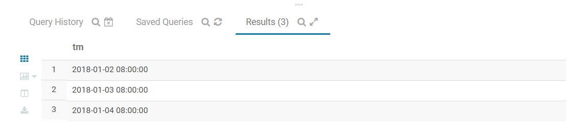
4.2.2.9 mysql 常用时间函数
current_date() -- now()
year(),week()
date_add(makedate(year(current_date()),1), interval week(current_date()) week)makedate(year(current_date()),1): 反馈当年第一天date_add(, interval ... week): 加上对应的天数,得到当星期的星期一
4.2.2.10 DATE_FORMAT的时间设定(mysql) (Oracle Corporation and/or its affiliates 2018a)
4.2.3 使用正则化提取变量
4.2.3.1 regexp_*
参考 S (2018) ,这是impala使用正则化一篇比较好的科普文,我整理了相关函数。
函数在R中的替换,
regexp_extract=str_extract- 注意
regexp_extract第三个参数是一定要有的,是取用第几个部分,这里的部分是需要用()括起来的。 - 后面的数字是 capture 的 portion
- 见 string 的第四章节
- 例子见 tutoring xumingde 的例子
- 注意
regexp_like=str_detect,反馈TRUE和FALSE!regexp_like(...,...)取反的快捷键
regexp_replace=str_replace
4.2.3.1.1 一些例子
> sqlQuery(impala,"select regexp_extract('10.0.1','(\\d{1,})',1)") %>% pull()
[1] 10
Warning message:
In strsplit(code, "\n", fixed = TRUE) :
  input string 1 is invalid in this locale
> # 这就将字段'10.0.1'第一个数字取出来了,{1,}表示大于等于1以上个数字
> sqlQuery(impala,"select regexp_replace('iPhone 6S Plus','[Ss]\\sPlus$','.75')") %>% pull()
[1] iPhone 6.75
Levels: iPhone 6.75
> sqlQuery(impala,"select regexp_replace('iPhone 6 Plus','\\sPlus$','.25')") %>% pull()
[1] iPhone 6.25
Levels: iPhone 6.25
> sqlQuery(impala,"select regexp_replace('iPhone 6s','s$','.5')") %>% pull()
[1] iPhone 6.5
Levels: iPhone 6.5
> # 这里假设一部iPhone 6和iPhone 6Plus手机差0.25的等级,iPhone 6和iPhone 6s差0.5的等级
> sqlQuery(impala,"select regexp_extract('iPhone 6.5','(\\d.\\d|\\d)',1)") %>% pull()
[1] 6.5
> # 这里就是把刚才的处理过的数据处理出来
解释
[[:alpha:]]: 大小写(CSDN博客 2017){1,}: 大小写一个以上\\)\\"\\]$: 分别表示一个)、"、]串联(Hopmans 2015)$: 按照以上形式结尾regexp_extract(col,0)取出变量col中第一个符合规则的字段regexp_replace(col,A,B)改变变量col中A部分的字段为B字段
select regexp_extract(phone_os_ver,'(\\d{1,})',1)
select regexp_replace(phone_model,'[Ss]\\sPlus$','.75')
select regexp_replace('iPhone 6 Plus','\\sPlus$','.25')
select regexp_replace('iPhone 6s','s$','.5')
select regexp_extract('iPhone 6.5','(\\d.\\d|\\d)',1)4.2.3.2 rlike
主要参考 Capriolo, Wampler, and Rutherglen (2012) 的书。
A RLIKE B, A REGEXP B
4.2.3.3 like和ilike的区别
like是大小写敏感的。ilike不是,其他功能类似。(Cloudera 2015b)
4.2.4 文本函数
4.2.4.1 split in Hive
在impala里面使用
split_part(string source, string delimiter, bigint n)
(Cloudera 2018c)。
4.2.4.2 合并文本 concat_ws
concat_ws(sep,s1,s2,...)
主要参考 Capriolo, Wampler, and Rutherglen (2012) 的书。
4.2.5 substr()函数
按照位置提取对应的文本。
在mysql中可以使用(Y. Du 2015)
substring(str, pos, length)
4.2.6 文本长度
select userid, substring(cast(userid as string),char_length(cast(userid as string))-1,char_length(cast(userid as string))) from xxx.test_50
4.2.6.1 身份证号里面取年龄
xxxs权限已禁用
with table_3 as
(
  with table_2 as
  (
    with table_1 as
    (
      select userid, idnumber,
      case
      when length(idnumber) = 18 then year(now())-cast(substr(idnumber,7,4) as decimal(20,0))
      when length(idnumber) = 15 then year(now())-cast(concat('19',substr(idnumber,7,2)) as decimal(20,0))
      end as age
      from xxxs.userdetails
    )
    select b.userid, b.mobile, a.age, a.idnumber
    from table_1 a
    right join [shuffle]
    test.gl201804_2 b
    on a.userid = b.userid
  )
  select
  -- userid, idnumber, age,
  case
    when age<=20 then '20-'
    when age>20 and age<=25 then '20-25'
    when age>25 and age<=30 then '25-30'
    when age>30 and age<=35 then '30-35'
    when age>35 and age<=40 then '35-40'
    when age>40 and age<=50 then '40-50'
    when age>50 then '50+'
    when age is null then 'xxxs.userdetails无身份证号'
    end as age_bin,
    count(1) as cnt
  from table_2
  group by 1
)
select age_bin, cnt
from table_3
order by 1length()识别长度substr取出生年月concat处理15位身份证号码
4.3 汇总函数 Aggregate functions
4.3.1 提取百分比及其运算 (Hive Only)
主要参考 Capriolo, Wampler, and Rutherglen (2012) 的书。
percentile(...,p1)比较慢。percentile(...,[p1,p2,..])(Hive only)histogram_numeric和collect_set目前还在debug
histogram_numeric(col, NB),比较慢。
x是bin值,y是count。
0.0和1.0不支持- 加上
array
with table_2 as
  (
    with table_1 as
      (select * from xxx.oprt_6_01_jx limit 100)
      select histogram_numeric(userid,3) as key_value_pairs
      from table_1
  )
  select key_value_pairs['x'], key_value_pairs['y']
  from table_2
这种key value pairs 我还不知道怎么取。
Hive 本身就是慢的,但是很多函数impala是没有的。
- Hive 的collect_set使用详解 - CSDN博客 实现上也有点鸡肋。
简化举例子
4.3.2 max、min和`null
max、min计算时忽略null,只有改列为空或者值全为空,才返回null
4.3.2.1 max默认null最小
4.3.2.2 min和max是剔除NULL去比较的
4.3.2.3 尽量保持无NULL
with table_1 as
(
select 1 as userid, NULL as success union all
select 2 as userid, 1 as success union all
select 3 as userid, 0 as success union all
select 4 as userid, 1 as success union all
select 5 as userid, 0 as success
)
select userid
from table_1
where success is not null如上面的代码,其实反馈的是success = 1 or success = 0的情况。
其实不需要保留success = 0,直接反馈success = 1的情况即可,这样表的大小缩减。
并且表不保存NULL,大大提高readability,方便直接left join
4.3.3 GROUPING SETS clause (Hive only)
The
GROUPING SETSclause in GROUP BY allows us to specify more than oneGROUP BYoption in the same record set. A blank set( )in the GROUPING SETS clause calculates the overall aggregate. (D. Du 2015)
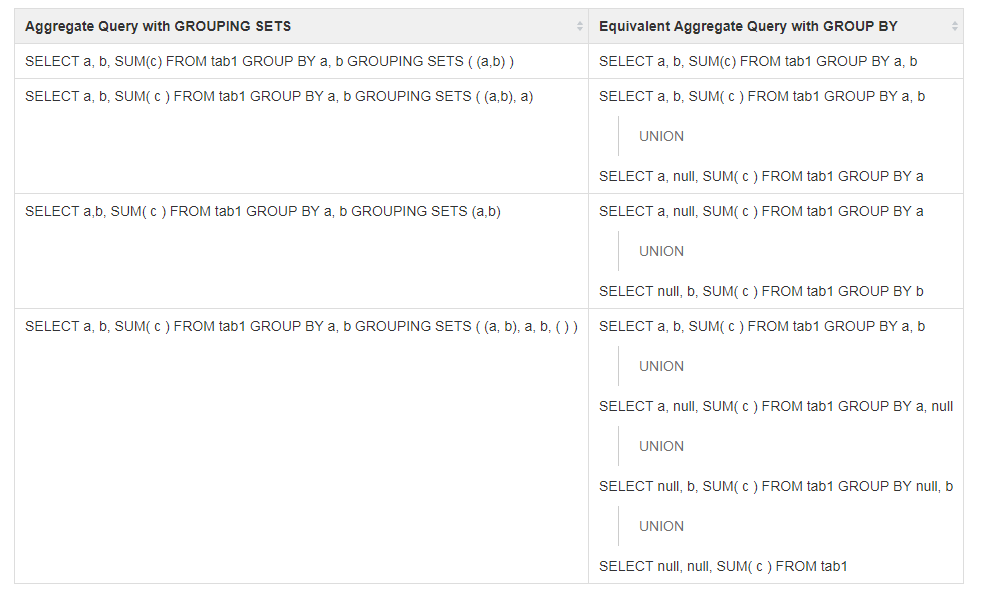
其实就是同一个set下,我们可以搞好几次group by,最后union。
WITH ROLLUP和
WITH CUBE无法使用。
4.3.4 补集
\[\complement_U A \bigcap \complement_U A = A \bigcup B\]
注意空集的情况。
4.3.5 count()注意的地方
distinct是不处理NULL的。
count(distinct x1,x2)等价于再加上条件where x1 is not null and x2 is not null,这是count的限制。
with table_1 as
(
  select NULL as x1, 1 as x2 union all
  select 1 as x1, 2 as x2 union all
  select 2 as x1, 3 as x2 union all
  select 3 as x1, 4 as x2 union all
  select 4 as x1, 5 as x2 union all
  select 5 as x1, NULL as x2 union all
  select NULL as x1, NULL as x2

)
select
count(distinct x1, x2)
from table_1

select
count(1),
count(distinct userid, amountsteptime),
sum(case when userid is null then 1 else 0 end) as not_null_cnt_userid,
sum(case when amountsteptime is null then 1 else 0 end) as not_null_cnt_amountsteptime
from table_4
4.3.5.1 多个count distinct的方式
cross join 过于复杂了
select v1.c1 result1, v2.c1 result2 from
  (select count(distinct col1) as c1 from t1) v1
    cross join
(select count(distinct col2) as c1 from t1) v2;- union all 是 long table 的展示形式
- subquery 是 wide table 的展示形式
library(DBI)
con <- dbConnect(RSQLite::SQLite(), ":memory:")
dbWriteTable(con, "mtcars", mtcars)
library(glue)
tbl <- "mtcars"| x1 |
|---|
| 25 |
| 3 |
参考 Khalil (2019, chap. 2 subquery)
select
    (select count(distinct mpg) as x1 FROM mtcars) as nunique_mpg
,(select count(distinct cyl) as x1 FROM mtcars) as nunique_cyl| nunique_mpg | nunique_cyl |
|---|---|
| 25 | 3 |
4.3.5.2 count(*) count(1) count(col) count(distinct col)的区别
with tbl_1 as
(
select 1 as x1, 2 as x2 union all
select 2 as x1, 3 as x2 union all
select 3 as x1, 4 as x2 union all
select 4 as x1, 5 as x2 union all
select 5 as x1, NULL as x2 union all
select NULL as x1, 6 as x2 union all
select NULL as x1, NULL as x2
)
-- select count(1) -- 7
-- select count(2) -- 7
-- select count(*) -- 7
-- select count(x2) -- 5
-- select count(x1, x2) -- 不能这样写
-- select count(distinct x1, x2) -- any NULL is eliminated
select distinct x1,x2 -- 不剔除样本
from tbl_1
The notation COUNT(*) includes NULL values in the total. (Cloudera, Inc. 2015)
count(1)count(2)count(*)
三者等价。
You can also combine
COUNTwith theDISTINCToperator to eliminate duplicates before counting, and to count the combinations of values across multiple columns. (Cloudera, Inc. 2015)
这个效果只有count和distinct一起使用时,才发生。
参考 Grant (2019)
count(*)- number of rowscount(column_name)- number of non-NULLvalues
因此
count(1)- 1非空,也是代表了 number of rows
4.3.5.3 count(False) = 1
with tbl_1 as
(
    select False as x1 union all
    select True as x1 union all
    select False as x1 union all
    select True as x1
)
select count(x1),sum(x1)
from tbl_1
-- 4 2count(False)= 1sum(False)= 0
4.3.5.4 正则化、count distinct 和 group by
with tbl_1 as
(
  select '101-345-5' as id union all
  select '101-345-6' as id union all
  select '101-345-6' as id union all
  select '102-345-5' as id union all
  select '101-345-5' as id union all
  select '103-345-8' as id union all
  select '103-345-8' as id
)
select
  substr(id,1,3) as cate, count(distinct id)
from tbl_1
group by 1
order by substr(id,1,3)这样不需要再创建一个cate变量,再with嵌套。
4.3.6 sum和条件
sum(prod_type=1 and status in (33,41,53,71,80,90,100)) 4.3.7 skewness 实现
参考 Michael (2014) 的想法,用R验证后无误。
sqlQuery(impala,"
with a as (
    with a as (
        select rand(1) as x1 union all
        select rand(2) as x1 union all
        select rand(3) as x1 union all
        select rand(4) as x1 union all
        select rand(5)
    )
    select x1, avg(x1) over () avg
    from a
)
select avg(pow(x1-avg,3))/pow(avg(pow(x1-avg,2)),1.5) as skewness
from a
         ")
# 0.2023669
R中验证结果相符。
library(tidyquant)
sqlQuery(impala,"
select rand(1) as x1 union all
select rand(2) as x1 union all
select rand(3) as x1 union all
select rand(4) as x1 union all
select rand(5)
         ") %>%
    summarise(skewness = skewness(x1))
# 0.2023669
4.3.7.1 Skewness undefined 的情况
假设一组数据\(C\),每个元素都为常数\(c\),
参考 Oloa (2017) 那么期望值、方差、峰度分别为
\[\begin{cases} \mathbb{E}(C)=c \\ \mathbb{Var}(C)=\mathbb{E}[(X-\mathbb{E}(X))^2] = \mathbb{E}(C^2)-(\mathbb{E}(C))^2=c^2-c^2=0 \\ \mathbb{Skew}(C)=\text{undefined} \\ \end{cases}\]
If all nonmissing arguments have equal values, the skewness is mathematically undefined. (SAS Documentation 2018, 1041)
常数的 skewness 是 undefined 的。(SAS Documentation 2018, 1041; Wikipedia contributors 2018b) 因为\(\mathbb{Var}(C)=0\)。
\[\begin{cases} \text{Symmetric distributions}\not\to \mathrm{skewness = 0} \\ \text{Symmetric distributions}\gets \mathrm{skewness = 0} \\ \end{cases}\]
注意的是,对称分布不代表skewness为0。
例如,
Cauchy distribution is symmetric, but its skewness isn’t 0. (“Skewness of a Random Variable That Have Zero Variance and Zero Third Central Moment,” n.d.)
柯西分布的重要特性之一就是期望和方差均不存在(undefined),因此skewness也是不存在的。(Wikipedia contributors 2018a)
针对 skewness undefined 的情况进行如下清洗。
一般来说,\(\mathrm{skewness \in [-1,1]}\),判断,
with a as (
    with a as (
        with a as (
            select  1 as x1, 1 as grp union all
            select  2 as x1, 1 as grp union all
            select  3 as x1, 1 as grp union all
            select  1 as x1, 2 as grp union all
            select  1 as x1, 2 as grp union all
            select  1 as x1, 2 as grp union all
            select  4 as x1, 3 as grp union all
            select  5 as x1, 3 as grp union all
            select  6 as x1, 3 as grp union all
            select 10 as x1, 4 as grp union all
            select 11 as x1, 4 as grp union all
            select 100 as x1, 4 as grp
        )
        select x1,grp
            ,avg(x1) over (partition by grp) avg
        from a
    )
    select
        avg(pow(x1-avg,3))/pow(avg(pow(x1-avg,2)),1.5) as skewness,grp
    from a
    group by grp
)
select
    case
        when is_nan(skewness)=1 then 'undefined'
        -- 这里将存在的值切分为2类,这个可以按照实际情况,增加到5-10类
        when skewness <= 0.5 then '[0,0.5]'
        when skewness  > 0.5 then '(0.5,1]'
        -- 定义other,只要是为了查证是否存在我们没有考虑到的情况
        else 'other'
        end
        as modified_skewness
    ,grp
from a
order by grp这里组grp=2的x1为常数,因此skewness 是 undefined。
4.4 取用每组最小时间数据的方法 mysql
inner join ( min ...)是取用group by最小时间的一种办法(Hislop 2011)。
4.5 分析函数 Analytic functions
Analytic functions are usually used with
OVER,PARTITION BY,ORDER BY, and the windowing specification.Function (arg1,..., argn) OVER ([PARTITION BY <...>] [ORDER BY <....>] [<window_clause>])(D. Du 2015, 章节6)
4.5.1 Function (arg1,..., argn)
rank: 排序dense_rank: 但是rank也会有重复值,但是全部是连续的。row_number(): 完全是按照order by来排序,注意这里的partition by是样本1。cume_dist: 小于等于目前这个值的样本比例。注意这个等于,决定了这里一定是\(\in (0,1]\)percent_rank: \(\frac{rank_{当前}-1}{rank_{总}-1}\)
WITH test
as
(
    select NULL as score
    UNION ALL
    select NULL
    UNION ALL
    select 10
    UNION ALL
    select 40
    UNION ALL
    select 40
    UNION ALL
    select 50
    UNION ALL
    select 50
    UNION ALL
    select 60
    UNION ALL
    select 90
    UNION ALL
    select 90
)
select
    ROW_NUMBER() over(order by score) as rownum
    ,score,cume_dist()over(order by score) as cum
    ,PERCENT_RANK() over(order by score) as per_rnk
    ,RANK() over(order by score) as rnk
from test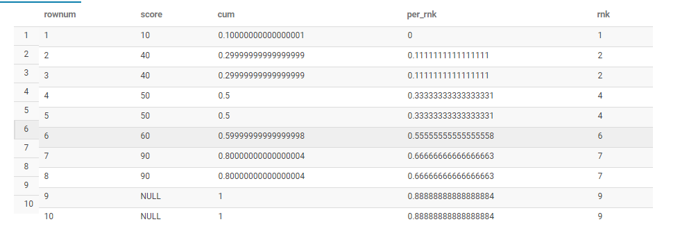
为什么空值最后计算,见 4.5.1.2。
参考: SQL SERVER中CUME_DIST和PERCENT_RANK函数 - CSDN博客
lead和lag:first_value和last_value: 类似于sql中的top 1
with table_1 as
(
  select borrowerid as userid, amount,
    cast(inserttime as timestamp) as inserttime
  from xxxlisting
)
select userid,
  lag(amount, 1) over (partition by userid order by inserttime) as amount_lag,
  lead(amount, 1) over (partition by userid order by inserttime) as amount_lead,
  first_value(amount) over (partition by userid order by inserttime) as amount_first,
  last_value(amount) over (partition by userid order by inserttime) as amount_last,
  last_value(amount) over (partition by userid order by inserttime rows between current row and 1 following ) as amount_last2
from table_1
4.5.1.1 row_number和where的先后顺序
row_number和where的先后顺序,或者说select和where的先后顺序。
显然是先 from 后 where 再 select 了。
4.5.1.2 设置NULL置前还是置后
There is no support for Nulls first or last specification. In Hive, Nulls are returned first (Bansal, Chauhan, and Mehrotra 2016)
ORDER BY col_ref [, col_ref ...] [ASC | DESC] [NULLS FIRST | NULLS LAST]这个可以设置,设置NULL置前还是置后。
with a as
(
    select 1 as x union all
    select 1 as x union all
    select 2 as x union all
    select null as x union all
    select null as x union all
    select null as x union all
    select 2 as x union all
    select 2 as x
)
select x
    ,row_number() over(order by x NULLS FIRST) as x1
    ,row_number() over(order by x NULLS  LAST) as x2
    ,row_number() over(order by x desc NULLS FIRST) as x3
    ,row_number() over(order by x desc NULLS  LAST) as x4
from ax1反馈NULL于1,2,3的位置,因为是asc排序, 然后让NULL最firstreturnx2反馈NULL于6,7,8的位置,因为是asc排序, 然后让NULL最lastreturnx3反馈NULL于1,2,3的位置,因为是desc排序,然后让NULL最firstreturnx4反馈NULL于8,7,6的位置,因为是desc排序,然后让NULL最lastreturn
Rows with a NULL value for the specified column are ignored. If the table is empty, or all the values supplied to AVG are NULL, AVG returns NULL.
avg()函数是不考虑NULL情况的。
反馈NULL的情况,也符合使用row_number的使用场景。
需要定义NULL置前还是置后。
4.5.1.2.1 时间变量验证
with tbl_2 as
(
    with tbl_1 as
    (
      select '2018-01-01 08:00:00' as tm union all
      select '2018-01-02 08:00:00' as tm union all
      select '2018-01-01 09:00:00' as tm union all
      select '2018-01-03 08:00:00' as tm union all
      select '2018-01-01 10:00:00' as tm union all
      select '2018-01-04 08:00:00' as tm union all
      select '2018-01-01 13:00:00' as tm union all
      select NULL as tm
    )
    select cast(tm as timestamp) as tm
    from tbl_1
)
select
    tm,
    row_number() over (order by tm) as row_num,
    last_value(tm) over (order by tm) as last_value,
    first_value(tm) over (order by tm) as first_value
from tbl_2
row_number依然判断NULL最大last_value有些奇怪
4.5.1.3 cumsum 功能 [Cloudera2018SUM]
with tbl_1 as (
    select 1 as x1, 1 as x2 union all
    select 2 as x1, 1 as x2 union all
    select 3 as x1, 1 as x2 union all
    select 4 as x1, 1 as x2 union all
    select 1 as x1, 2 as x2 union all
    select 2 as x1, 2 as x2 union all
    select 3 as x1, 2 as x2 union all
    select 4 as x1, 2 as x2
)
select x1,x2
  ,sum(x1) over (partition by x2 order by x1) as 'cumulative total'
from tbl_1
4.5.2 [PARTITION BY <...>] s
类似于group by
4.5.3 [ORDER BY <....>]
类似于order by
4.5.4 [<window_clause>]
最后function的数据范围,是current row的前多少后多少可以满足。
rows between current row and 1 followingrows between 2 preceding and current rowrows between 2 preceding and unbounded followingrows between 1 preceding and 2 precedingrows between unbounded preceding and 2 preceding
If we omit BETWEEN…AND (such as
ROWS N PRECEDINGorROWS UNBOUNDED PRECEDING), Hive considers it as the start point, and the end point defaults to the current row. (D. Du 2015)
在使用partition by求汇总量时,和group by求汇总量是不同的。
如果其中没有加入window函数,那么这里是默认求解排序后第一行到当前行的汇总量,并非是排序后第一行到最后一行的汇总量。
4.5.4.1 举例
举一个例子,如下面这段code,
last_value(y) over (partition by x order by y) as last_value1隐含了BETWEEN UNBOUNDED PRECEDING AND current row,也就是从当前行和之前的行中求最后一行。first_value(y) over (partition by x order by y) as first_value1隐含了BETWEEN UNBOUNDED PRECEDING AND current row,也就是从当前行和之前的行中求最前一行。当然这也是我们需要的结果,但是只是一个巧合。
我们真正需要的是last_value2和first_value2,也就是每个 partition 的子表内,当前行前面所有行和后面所有行内求last_value和first_value。
因此按照实际业务需求来说,我们使用时,应该加上ROWS BETWEEN UNBOUNDED PRECEDING AND UNBOUNDED FOLLOWING。
with a as
(
  select 1 as x, 1 as y union all
  select 1 as x, 2 as y union all
  select 1 as x, 3 as y union all
  select 1 as x, 4 as y union all
  select 2 as x, 1 as y union all
  select 2 as x, 2 as y union all
  select 2 as x, 3 as y union all
  select 2 as x, 4 as y
)
select
    x,y
    ,last_value(y)  over (partition by x order by y) as  last_value1
    ,first_value(y) over (partition by x order by y) as first_value1
    ,last_value(y)  over (partition by x order by y ROWS BETWEEN UNBOUNDED PRECEDING AND UNBOUNDED FOLLOWING) as  last_value2
    ,first_value(y) over (partition by x order by y ROWS BETWEEN UNBOUNDED PRECEDING AND UNBOUNDED FOLLOWING) as first_value2
    ,last_value(y)  over (partition by x order by y ROWS BETWEEN UNBOUNDED PRECEDING AND current row) as  last_value3
    ,first_value(y) over (partition by x order by y ROWS BETWEEN UNBOUNDED PRECEDING AND current row) as first_value3
from a
因此,修改后的代码为,
4.5.4.2 R 实现例子的代码
library(data.table)
library(lubridate)
tst_lastvalue <-
data.table(
    id = 1:100
    ,user_id = 1:10
) %>%
    mutate(t = today() + ddays(id)) %>%
arrange(user_id,t)sqlDrop(impala,'xxx.tst_lastvalue_xxx')
tst_lastvalue %>%
group_by(user_id) %>%
mutate(last_t = max(t)) %>%
mutate_if(is.Date,as.character) %>%
sqlSave(channel = impala,dat = .,tablename = 'xxx.tst_lastvalue_xxx',rownames=FALSE,addPK = FALSE)时间需要文本化。
使用last_value()函数取出last_t列就好。
4.5.5 define window function (Hive 慢)
4.6 集合函数 table generating functions
4.6.1 Hive From 嵌套表
nested subquery in Hive (Capriolo, Wampler, and Rutherglen 2012, 113)。
FROM (
SELECT * FROM people JOIN cart
ON (cart.people_id=people.id) WHERE firstname='john'
) a SELECT a.lastname WHERE a.id=3;
Hive只支持在FROM子句中使用子查询,子查询必须有名字,并且列必须唯一。
4.6.2 explode函数
hive> SELECT array(1,2,3) FROM dual;
[1,2,3]


hive> SELECT explode(array(1,2,3)) AS element FROM src;
1
2
3
类似于R dplyr::gather函数。
(Capriolo, Wampler, and Rutherglen 2012, 164)
这里别忘记split函数,否则会报错。
因为explode不接受list。
Error while compiling statement: FAILED: UDFArgumentException explode() takes an array or a map as a parameter4.6.3 lateral view函数
hive> SELECT name, explode(subordinates) FROM employees;
FAILED: Error in semantic analysis: UDTF's are not supported outside
the SELECT clause, nor nested in expressions

hive> SELECT name, sub
> FROM employees
> LATERAL VIEW explode(subordinates) subView AS sub;
John Doe    Mary Smith
John Doe    Todd Jones
Mary Smith  Bill King
但是当explode和其他变量一起存在select statement中时,会报错,这时需要放入
LATERAL VIEW并给予命名subView,和其变量的命名sub,命名可直接在select中使用。
(Capriolo, Wampler, and Rutherglen 2012, 165)
LATERAL VIEW 实现gather的效果。(Francke and Apache Software Foundation 2013)
select myCol1, myCol2
from
(
    select array(1,2) as col1, array("a", "b", "c") as col2 union all
    select array(3,4) as col1, array("d", "e", "f") as col2
) a
LATERAL VIEW explode(col1) myTable1 AS myCol1
LATERAL VIEW explode(col2) myTable2 AS myCol2;from不能前置。

4.6.4 get_json_object函数
-- Hive

create table xxx.seekingxxx_xxx_jx as
select name_02
from
(
    from
    (
        from
        (
            select uuid, get_json_object(app_infos, "$.appInfos.name") as col_01 from
            xxxxxx_app_info_list
        ) a
        select name_02
        LATERAL VIEW explode(split(col_01, '","')) subView AS name_02
        group by name_02
    ) b
    select regexp_replace(name_02, '\\["',"") as name_02
    group by regexp_replace(name_02, '\\["',"")
) c;

-- impala

INVALIDATE METADATA xxx.seekingxxx_xxx_jx;
compute stats xxx.seekingxxx_xxx_jx;

-- rename

alter table xxx.t180606_prodxxxxxx_xxx rename to xxx.t180606xxxxxx_AppList_xxx;- 业务需求: 从所有App中,确认查询App是否在表
xxxxxx_app_info_list中。 - 命名解释:
[创建时间]_[业务线]_[内容]_[Owner],参考 Bryan (2018a), Bryan (2018b)。 explode函数见 4.6.2lateral view4.6.3get_json_object函数见 4.6.4- 先执行
INVALIDATE METADATA,后执行compute stats,注意是在impala中执行这两条代码。 rename函数参考 1.9regexp_replace函数参考 4.2.3,[剔除,输入\\[,参考 Bergquist (2014)。- Hive
From嵌套表参考 4.6.1 get_json_object是Hive函数,应该在Hive中使用。$表示根目录(Root object).表示子操作连接符(Child operator),更多参考 Sherman and Apache Software Foundation (2017)。
get_json_object(STRING json, STRING jsonPath)
A limited version of JSONPath is supported ($ : Root object, . : Child operator, [] : Subscript operator for array, * : Wildcard for []- 变量
app_infos下的 - Key
appInfos的value中 - 所有Key
name的value,建立一个list在一个单元格 - 最后变量命名为
col_01
5 数据表描述 describe
5.1 取得impala表的信息,如owner
sqlQuery(impala,'describe formatted xxx.test_cjf000') %>%
  filter(name %in% str_subset(name, "Owner")) %>%
  select(type) %>%
pull()我们发现在owner行,type列中。
5.2 使用map2批量操作
a <- sqlTables(impala,schema = 'xxx')sqlTables可以批量读取一个库的所有表的汇总信息,这里是为了提取表名,用于for循环。
getowner <- function(a,b){
  sqlQuery(impala,str_c('describe formatted ',a,".",b)) %>%
  filter(name %in% str_subset(name, "Owner")) %>%
  select(type) %>%
  pull()
}
a %>%
select(2:3) %>%
head() %>%
mutate(owner = map2(TABLE_SCHEM,TABLE_NAME,getowner)) %>%
unnest()批量输出owner的方式。
5.3 describe (…) tablename
主要参考 Capriolo, Wampler, and Rutherglen (2012) 的书。
creator这些信息都可以查到。location:hdfs://hdpha/user/hive/warehouse/xxx.db/ln_hive_jx- 内存为0的情况是因为未
compute stats
5.4 查看sql使用了那些表
get_db_table <- function(x){
db_name <-
c("ddm","default","edw","erp","ext","mdl_data","xxxquot;,"xxxv","xxx","test","tmp","xkyy")
db_name_edited <- paste("(",paste(db_name,collapse = "|"),")",sep="")
read.table(x, sep="\t") %>%
mutate(table = str_extract(V1,paste(db_name_edited,"\\.[:graph:]{5,}",sep="")),
       table = str_remove(table,";|\\)")) %>%
  filter(!is.na(table)) %>%
  distinct(table) %>%
  mutate(database = str_extract(table,"[[:lower:]_]{3,7}\\."),
         database = str_remove(database,"\\.")) %>%
  select(database,table)
}
5.5 百分号和星号的区别
我提了一个问题在Stack Overflow上,讨论百分号和星号的区别。 百分号和星号两者功能类似(Stack Overflow 2009),但是在不同的statement中有限制。
*只能在showstatement中使用里面执行 (Cloudera 2015a)%只能在selectstatement 这些查询语句里面 (Ellingwood 2013)show databases ‘a’; show databases like ’a’; show tables in some_db like ‘fact’; use some_db; show tables ‘dim|fact’;
因此%在show statement中执行是无效的。
The percentage sign (%) is used as the “everything” wildcard instead of an asterisk. It will match zero or more characters. (Ellingwood 2013)
5.6 查询版本信息 (DuBois 2014, 151)
SELECT USER(), CHARSET(USER()), COLLATION(USER())
,VERSION();USER()CHARSET(USER())\tCOLLATION(USER())\tVERSION()`utf8utf8_general_ci\tread_ayokredit@10.1.32.209\t5.7.19-17-log`
6 R
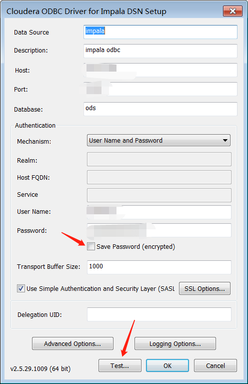
6.1 R连接impala
参考这篇
Manual
下载安装ClouderaImpalaODBC64.msi,如果系统是32位,下载对应的ClouderaImpalaODBC32.msi。
Cloudera, Inc. (2014) 的教程写的过于复杂。
开始打开64-bit ODBC Administrator- 在老邻居
Excel旁边点击impala - 修改配置,
Host改为10.2.8.98 - 点击
OK - 重新在R里面配置impala就好了
有时候服务器很卡出现
> con <- odbcConnect('Impala')
[RODBC] ERROR: state HY000, code 3, message [Cloudera][ThriftExtension] (3) Error occurred while contacting server: ETIMEDOUT. The connection has been configured to use a SASL mechanism for authentication. This error might be due to the server is not using SASL for authentication.ODBC connection failed这时候换下Host的名字就好了,比如10.2.8.98改为10.2.8.99,
\(99 \to 105\)都可以尝试一下。
另外记得认证,选中
\(\checkmark\)Use Simple Authentication and Security Layer (SASL)

6.2 重要的dependency包
# library(RODBC)
# impala <- odbcConnect("Impala")
library(tidyverse)
library(lubridate)
library(knitr)
{r message=FALSE, warning=FALSE, include=FALSE}主要不报错。因为很多。RODBC包是书写sql的。tidyverse是主要处理数据,dplyr(mutate,arrange),tidyr(gather,spread),%>%用得最多。knitr导出格式,一般是kable\(\to\)knit table \(\to\) 编织表格。cache=T如果执行过,产生图片、数据,用电脑临时存储的。- 英文输入法环境下,
ctrl+shift+K\(\to\) 产生一个输出格式,.html。 你可以再修改.Rmd后,重复使用。 但是每次点击的时候,sql都是要重新执行一遍。
6.3 R里面传数据到impala
sqlSave(impala, vars_name, tablename='xxx.vars_name',
rownames=FALSE, addPK=FALSE)sqlQuery是下载数据,那么
sqlSave就是上传数据。
其中impala是接口,大家都知道。
vars_name是R中我们队数据表得命名,
tablename='xxx.vars_name'是我们想在impala库中给予的命名,
rownames=FALSE表达了我们的列有名字,不需要重命名。
以后就不用.csv文件上传数据了。
但是经常报错,目前没有很好的解决方案。
6.4 R 翻译到 SQL
## <SQL>
## SELECT `x`, AVG(`y`) AS `z`
## FROM `df`
## GROUP BY `x`
没有显示 code,但是在 console 里面会显示。
> df1 %>%
+   group_by(x) %>%
+   summarise(z = mean(y))
<SQL>
SELECT `x`, AVG(`y`) AS `z`
FROM `df`
GROUP BY `x`
Warning message:
Missing values are always removed in SQL.
Use `mean(x, na.rm = TRUE)` to silence this warning
This warning is displayed only once per session. ## <SQL>
## SELECT *
## FROM `df`library(tidyverse)
library(dbplyr)
mtcars %>%
dbplyr::tbl_memdb() %>%
group_by(cyl) %>%
filter(disp > mean(disp))
# Window function `MIN()` is not supported by this database
# Error: Window function `AVG()` is not supported by this database
# 但是 mean 其实在官方链接里面用了
# https://www.tidyverse.org/articles/2019/04/dbplyr-1-4-0/
# 看来要用 avg(xxx) over()6.5 sqlQuery中活用paste函数
data<-RODBC::sqlQuery(myconn,
paste("select * from table
        where create_time between between to_date('", format(Sys.Date()-1,'%Y%m%d'), " 00:00:00', 'yyyymmdd hh24:mi:ss')
        and to_date('", format(Sys.Date()-1,'%Y%m%d')," 23:59:59', 'yyyymmdd hh24:mi:ss')",
sep="")paste函数,这里有用。
6.6 下载速度
data <-
sqlQuery(impala,"select insertmonth,regchanel,count(*) cnt
from (
select userid,inserttime,regchanel,device,sourcename,substr(cast(inserttime as string),1,7) insertmonth
from xxx.userregsource_md
where inserttime>'2017-06-01'
) b
group by insertmonth,regchanel;")- 这个是一个sql的模版。
- 输入量很大,因此记得加
limit,看看数据。 - <30万,下载时间在1min,按照现在集群的正常水平。
count(1)可以提前查询表的大小。为什么用count(1),因为count可能不记录缺失值。- 如果不单执行,
create table正常用,不用担心,这只是传命令到impala。
6.7 导出str,防止转成数字
sqlQuery()函数中as.is = TRUE参数(Marquez 2017),保证了str格式的字段不会转换成其他格式。mutate_all(.funs = ~paste0("'",.))保证了write_excel_csv写入str不会自动转换成数字。
6.8 实现 Impala 的 for 循环
这里限定变量类型是因为 impala 会自动修改类型,因此工程上为了误差小,这里限定。 参考issues。
insert overwrite xxx.t190203_test_forloop_xxx
select cast(x1 + 1 as smallint) as x1
from xxx.t190203_test_forloop_xxx这里完成了一次循环,因此以下可以进行十次测试。
library(RODBC)
impala <- odbcConnect("Impala")
# restart
sqlQuery(impala,"
insert overwrite xxx.t190203_test_forloop_xxx
select cast(100 as smallint) as x1
         ")
for (i in (1:10)) {
    sqlQuery(impala,"
    insert overwrite xxx.t190203_test_forloop_xxx
    select cast(x1 + 1 as smallint) as x1
    from xxx.t190203_test_forloop_xxx
             ")
}同样地,while 和 repeat 可以在 R 中调用也可以实现。 思路参考fronkonstin
6.9 批量执行 SQL
目前函数的功效是能够在 Impala 在跑类似于 insert overwrite 等,反馈报错。
任何需要前置的 library 的包 或者自定义函数,提前在一个 config 文件完成就好,然后 source 的时候前置即可。
如在执行 .R 文件内,写入
文件 impala_in_r.R 便是 config 文件。
目前,
write_job.R 针对于 sql 文件,可以输出 R 或者 Python 格式的文件。
目前有sample.sql,
library(xfun)
library(tidyverse)
library(glue)
read_utf8("sample.sql") %>%
    str_flatten("\n") %>%
    cat
## -- first example
##
## select 1 as x1
##
## -- second example
##
## select 1 as x1
##
## -- first example for insert
##
## insert overwrite xxx.test_insert_table_warning_xxx
## select 1 as x1通过函数write_job,见write_job.R,创建可以在 R 中执行的脚本。
## library(RODBC)
## impala <- odbcConnect('Impala')
## safely_run_impala("
## insert overwrite xxx.test_insert_table_warning_xxx
## select 1 as x1")
## safely_run_impala("
## select 1 as x1
## ")
## safely_run_impala("
## select 1 as x1
## ")
需要加载 config 文件,见impala_in_r.R,
最后执行source-test.R,即可。
## source("impala_in_r.R",encoding = "UTF-8")
## source("sample.R",encoding = "UTF-8")
点击 run job
当代码中存在 insert overwrite 报错时,会出现以下结果。
library(knitr)
include_graphics(here::here("analysis/safely-run-impala/figure/func-return-warning.png"))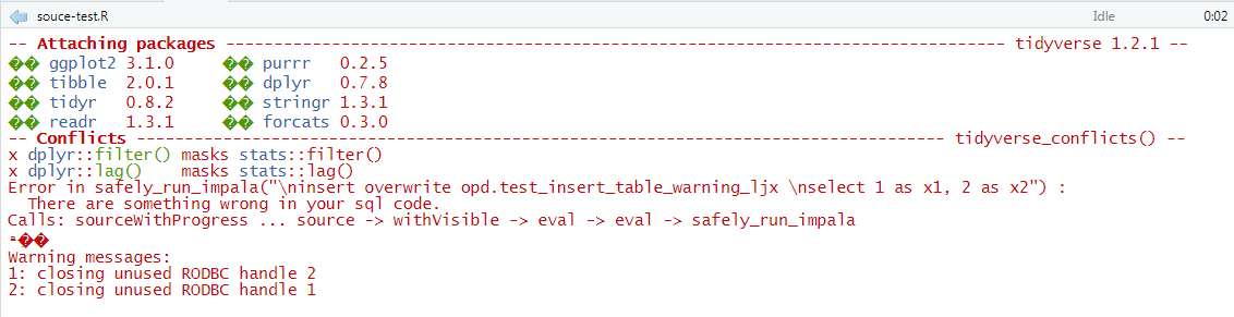
6.10 mutate + sum using SQL
参考 Pernes (2019)
可以用于标准化,加入 avg 和 std。
6.11 使用 R 批量执行 Impala 代码步骤
6.11.1 文件夹的构造
保存好自己需要执行的 SQL 代码。 拆分 SQL 代码,构建参考文件夹的构造,一个文件内理论上只能有一个建表、读表逻辑。
 把SQL文件上传到指定位置。
6.11.2 使用 Merge Request
把SQL文件上传到指定位置。
6.11.3 安装 R 和 RStudio
按照要求安装好 R 和 RStudio,必要的包。
R是底层软件,RStudio是使用它比较方便的软件,界面友好。
6.11.3.1 安装R
- 打开网址The Comprehensive R Archive Network
- 选择Download R for Windows
- 选择install R for the first time
- 选择Download R 3.x.x for Windows。
- 然后点开对应的
.exe文件,安装好。
6.11.3.2 RStudio
- 打开网址RStudio – Open source and enterprise-ready professional software for R
- 下载RStudio,Shiny和R Packages两个暂时不用管。
- 选择Free的第一个Download RStudio – RStudio。
- 然后点开对应的
.exe文件,安装好。 - 安装好了,就可以开始最简单的录入,EDA等等简单,后面再搞回归那些R弄起来都很简单,有现成的包。
6.11.3.3 安装重要的包
打开 RStudio
右上角,点击新建项目,选路径,选新项目。 给名字(不要中文),点击 Create Proj \(\to\) Tools \(\to\) Global Options \(\to\) Packages \(\to\) Mirror \(\to\) 选一个中国的镜像,选清华
安装包 点
- Tools \(\to\) Install Packages \(\to\) ‘tidyverse’ \(\to\) Install
- Tools \(\to\) Install Packages \(\to\) ‘rebus’ \(\to\) Install
- Tools \(\to\) Install Packages \(\to\) ‘rmarkdown’ \(\to\) Install
左上角
R Notebook \(\to\) 新建一个Rmd \(\to\) Ctrl + S Save
快捷键 Ctrl + Alt + I 新建 chunk
快捷键 Shift + Ctrl + Enter run
再新建一个 Chunk Ctrl + Alt + I
6.11.4 执行 R Job
参考 McPherson (2019)
When you run an R script in RStudio today, the R console waits for it to complete, and you can’t do much with RStudio until the script is finished running.
正是我的痛点,现在 Jobs 这个功能解决了。
同时已经封装到 rstudiapi 包中。
更快的方式是使用函数jobRunScript {rstudioapi}
## function (path, name = NULL, encoding = "unknown", workingDir = NULL,
##     importEnv = FALSE, exportEnv = "")
## NULL此时会直接调用到 Jobs 窗口。
6.11.5 代码优化
批量执行的代码,直接跑动,参考
library(magrittr)
if (!sessioninfo::os_name() %>% stringr::str_detect("Ubuntu")) {
setwd(here::here())
} else {
setwd("/home/jiaxiang/Documents/xxx")
}


source(here::here("R/batch-process-xxx-01.R"), encoding = "UTF-8")

system("git add .")
system("git commit -m 'Task #68 daily runs, track it. @xxx xxx'")
system("git push")
代码优化,包括打印日志、报错信息等参考
run_impala <-
function(file_path,
         log_path = here::here("output/xxx/running-log.md")) {
    text <- read_file(file_path)
    lines <- read_lines(file_path)[1:5] %>% na.omit()
    lines <- lines %>% str_flatten("\n")

    # run_sql <-
    # if (!sessioninfo::os_name() %>% str_detect("Ubuntu")) {
    #     purrr:partial(sqlQuery, channel = impala)
    # } else {
    #     purrr::partial(dbGetQuery, conn = con)
    # }
    # results <- run_sql(text)
    results <-
        if (!sessioninfo::os_name() %>% str_detect("Ubuntu")) {
            safely(sqlQuery)(impala, text)
        } else {
            safely(dbGetQuery)(con, text)
        }
    glue(
        "
     ###########################################################################
     # {basename(file_path)} runs at {Sys.time() %>% as.character()}                             #
     ###########################################################################
     at {dirname(file_path)}
     "
    ) %>% print
    # if (results == character(0)) {
    #     print('run successfully!')
    # } else {
    #     print(results)
    # }
    print(results)
    results <-
        results %>%
        unlist() %>%
        str_remove_all("^\\s+") %>%
        str_flatten("\n")
    append_content <- glue("# {basename(file_path)} {Sys.time()}
\```sql
{results}
\```
                       ")

    c(append_content, read_lines(log_path)) %>% write_lines(log_path)

    ui_warn("The error log is saved in the path") %>% print
    ui_path(log_path) %>% print
}
7 Python
7.1 Python连接impala
代码参考 Notebook
打开 Anaconda Prompt 安装 dependency 包(impyla,thrift_sasl,pure-sasl)。
每次conda和pip时,win7的python一定会说命令提示符提示不是内部或外部命令,需要设置环境变量再重启。
注意这个地方,thrift模块有版本限制,不然会报错。
使用conda list查询thrift版本。
用pip uninstall thrift卸装,
用pip install thrift==0.9.3按照这个老的版本。
在 Notebook 中,
conn = connect(host='xxx', auth_mechanism='PLAIN', port=xxx, user='xxx', password='xxx')
书写正确的信息,在生产中不要把明文密码写入。
下面是一段测试的代码。
runing sql @ 1[0.05, 0.1, 0.15, 0.2, 0.25, 0.3, 0.35, 0.4, 0.45]不然反馈的是整数。
使用 Python 连接 Impala。
8 表达 statement
表达,便非函数。
8.1 Queries that Sample Data (Hive Only)
主要参考 Capriolo, Wampler, and Rutherglen (2012) 的书。
这样不需要order by rand(123),因为order by很耗时间。
8.2 case when
8.2.1 sql批量打case when
借助excel,例如,
when profit <= -2050 then -2050。
打好case,
前一个单元格键入
when x <=,
右边value,
右边then,
右边value,
然后粘贴到visual code里面。
8.2.2 判断条件、if、case when 和空值处理
with a as (
    select 1 as x1 union all
    select 2 as x1 union all
    select null as x1
)
select
    -- sum
    sum(x1 = 1) as sum_wether,
    sum(if(x1 = 1,1,0)) as sum_if,
    sum(case when x1 = 1 then 1 else 0 end) as sum_case_when,

    -- avg
    avg(x1 = 1) as avg_wether,
    avg(if(x1 = 1,1,0)) as avg_if,
    avg(case when x1 = 1 then 1 else 0 end) as avg_case_when

from a

-- if 和 case when 是没有问题的,但是直接的判断条件会剔除null
-- 所以要简化 case when 用 if()| sum_wether | sum_if | sum_case_when | avg_wether | avg_if | avg_case_when |
|---|---|---|---|---|---|
| 1 | 1 | 1 | 0.5 | 0.3333333 | 0.3333333 |
8.2.3 简化 case when null 的代码
with tbl as
(
    select 1 as x1 union all
    select 1 as x1 union all
    select 1 as x1 union all
    select 1 as x1 union all
    select 1 as x1 union all
    select NULL as x1
)
select
    if(x1 is null, 'null', 'notnull') as x2
    ,x1 is null as x3
    ,x1
from tbl
比 case when好在不会因为忘记end报错而降低效率。
下面是直接覆盖值的方法
with tbl as
(
    select 1 as x1 union all
    select 1 as x1 union all
    select 1 as x1 union all
    select 1 as x1 union all
    select 1 as x1 union all
    select NULL as x1
)
select isnull(x1, -999) as x2, x1
from tbl
with tbl as
(
select 1 as x1 union all
select 1 as x1 union all
select 1 as x1 union all
select 1 as x1 union all
select 1 as x1 union all
select NULL as x1
)
select ifnull(x1, -999) as x2, x1
from tblisnull和ifnull一致。
8.2.4 case when 的 else
select
    1 > null
    ,case when 1>null then 1 else 0 end
    ,case when 1>null then 1 when 1<=null then 0 else -1 end
    ,istrue(1 > null)

null, 0, -1, false不一样的原因是else 是0,那么else包含了null的情况。
也就是说,1 > null这种判断条件,会受到干扰,有null时,用case when的else来处理。
istrue的false包含了null情况。
8.3 on vs. using
MySQL 在使用on条件时,可以用using简化。
(My SQL Tutorial 2018)
9 using (var)
on a.var = b.var9.1 WITH Clause (Cloudera, Inc. 2018g)
Many Data Analysts and Data Scientists prefer
WITHstatements to nestedFROMstatements because it’s easier to for a third party to review the query and to follow the logic of the original coder. (Green-Lerman 2018)
WITH语句方便第三方去检查code。
因此大家应该舍弃
TEMPTables 和- Nested
FROMstatements
的表达。
又叫 subquery factoring
with
t1 as (
    select 1
),
t2 as (
    select 2
    )
select *
from t1
union all
select *
from t2;
SQL code that is easier to read and understand by abstracting the most complex part of the query into a separate block. (Cloudera, Inc. 2018g)
这是优点之一。
with
t1 as (
    select 1 as x1
),
t2 as (
    select 1 as x2
    )
select *
from t1
inner join [shuffle] t2
on t1.x1 = t2.x2;
join 也可以执行。
9.1.1 with表可以在内嵌表中调用
with a as (
select 1 as x1
)
select x1
from (select x1 from a) b
这个应该有启发,但是具体如何实现,还要再看看。
9.2 Subqueries in HAVING clause (DuBois 2014, 298)
SELECT
    COUNT(1) as cnt,
    left(cast(user_id as CHAR(50)),1) as name
FROM tb_u_basic_info
GROUP BY name
having cnt = (
    select count(1)
    from tb_u_basic_info
    group by left(cast(user_id as CHAR(50)),1)
    order by count(1) desc
    limit 1
)
AnalysisException: Subqueries are not supported in the HAVING clause.但是impala中不能执行。
9.3 group by x不报错无影响
如代码,group by 1加不加都没有影响。
group by 1,2,3在mysql里面不能识别,因此会出现只出现一条数据的问题。
也就是说impala应该进行group by在mysql中未执行。
9.4 虚拟分RAND()实现
with a as (
    select id, FLOOR(1 + (RAND() * 3)) as gp
    from tb_loan_debt
    limit 10000
)
select count(1), gp
from a
group by gp
order by gp
虚拟分也可在impala中实现。
select cnt,gp
from (
select count(1) as cnt, FLOOR(1 + (RAND(1) * 3)) as gp
from tb_loan_debt
) a
group by gp
FLOOR(i + RAND() * (j − i)表示一个随机整数R在区间\(i \leq R \leq j\)(Oracle Corporation and/or its affiliates 2018c; w3resource.com 2018)。
duplicate entry 1 for key <group_key>
o
RAND()不能进group by和order by,即使是嵌套的方式也不可以(Milivojevic and Dubois 2016)。
9.5 Subqueries in Impala SELECT Statements (Cloudera, Inc. 2018f)
9.5.1 scalar subquery
SELECT x FROM t1 WHERE x > (SELECT MAX(y) FROM t2);就是用一个标量
9.6 WITH ROLLUP (DuBois 2014, 300)
SELECT
    COUNT(1) as cnt,
    left(cast(user_id as CHAR(50)),1) as name
FROM tb_u_basic_info
GROUP BY name WITH ROLLUP
WITH ROLLUP会再最后再加入一个汇总量
9.7 histogram图 (DuBois 2014, 518)
SELECT
    COUNT(1) as cnt
    ,REPEAT('*',round(COUNT(1)/10000)) AS histogram
    ,left(cast(user_id as CHAR(50)),1) as name
FROM tb_u_basic_info
GROUP BY name WITH ROLLUP
\(\Box\) 没有跑成功 \(\Box\) 占比再尝试
附录
9.8 Overview of the Hadoop ecosystem
knitr::include_graphics("https://raw.githubusercontent.com/JiaxiangBU/picbackup/master/hadoopeccosystem.png")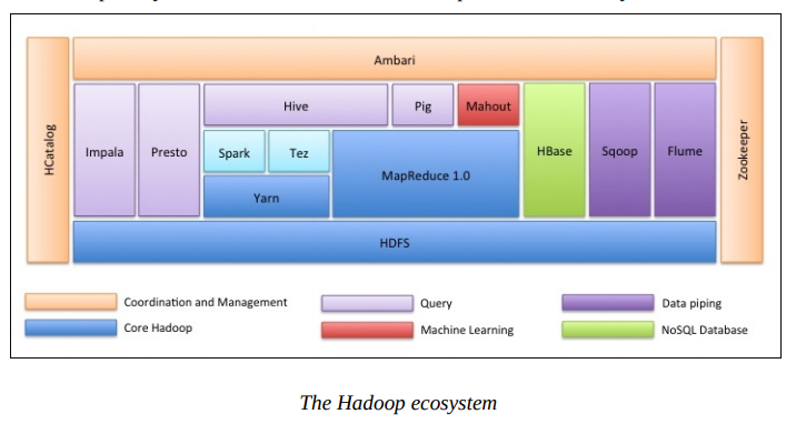
Figure 9.1: Hadoop 生态体系
9.9 数据类型
9.9.1 文本
参考 DataCamp chapter 2 ,但是学到的很少。
varchar [ (x) ]: (varying n) a maximum of n characterschar [ (x) ]: a fixed-length string of n characters
9.9.2 数字
参考 Grant (2019, chap. 2)
decimal/numeric可以表达更精确的数据。
9.9.3 时间
ISO 8601,参考 Grant (2019, chap. 4)
- ISO = International Organization for Standards
- YYYY-MM-DD HH:MM:SS
- Example: 2018-01-05 09:35:15
UTC = Coordinated Universal Time
- Timestamp with timezone:
- YYYY-MM-DD HH:MM:SS+HH
- Example: 2004-10-19 10:23:54+02
## SELECT rand(1) as x1 union all
## SELECT rand(2) as x1 union all
## SELECT rand(3) as x1 union all
## SELECT rand(4) as x1 union all
## SELECT rand(5) as x1 union all
## SELECT rand(6) as x1 union all
## SELECT rand(7) as x1 union all
## SELECT rand(8) as x1 union all
## SELECT rand(9) as x1 union all
## SELECT rand(10) as x1 union all
因为限定了状态,因此rand可以进行重复试验。
参考Blog
利用 cume_dist 可以进行对打分进行实时的标准化打分。
WITH a as (
    SELECT rand(1) as x1 union all
    SELECT rand(2) as x1 union all
    SELECT rand(3) as x1 union all
    SELECT rand(4) as x1 union all
    SELECT rand(5) as x1 union all
    SELECT rand(6) as x1 union all
    SELECT rand(7) as x1 union all
    SELECT rand(8) as x1 union all
    SELECT rand(9) as x1 union all
    SELECT rand(10) as x1
)
select
    x1
    ,(x1 - min(x1) over())
        /(max(x1) over() - min(x1) over())
    as x_normalized
    ,cume_dist() OVER(order by x1) as x1_pctg
    ,round(cume_dist() OVER(order by x1)*10,0) as x1_rating
from a 9.11 EXPLAIN 用法
参考 Russell (2014)
You can see the results by looking at the EXPLAIN plan for a query, without the need to actually run it
不需要实际执行。
To understand the flow of the query, you read from bottom to top. (After checking any warnings at the top.) For a join query, you prefer to see the biggest table listed at the bottom, then the smallest, second smallest, third smallest, and so on.
先看 warnings,再看 join 里的大表情况。
9.11.1 设变量优化
[localhost:21000] > explain select count(*) from partitioned_normalized_parquet
> join stats_demo_parquet using (id)
> where
> substr(partitioned_normalized_parquet.name,1,1) = 'G';
+-------------------------------------------------------------------------+
| Explain String                                                                            |
+-------------------------------------------------------------------------+
| Estimated Per-Host Requirements: Memory=194.31MB VCores=2                                 |
|                                                                                           |
| 06:AGGREGATE [MERGE FINALIZE]                                                             |
| | output: sum(count(*))                                                                   |
| |                                                                                         |
| 05:EXCHANGE [UNPARTITIONED]                                                               |
| |                                                                                         |
| 03:AGGREGATE                                                                              |
| | output: count(*)                                                                        |
| |                                                                                         |
| 02:HASH JOIN [INNER JOIN, BROADCAST]                                                      |
| | hash predicates: oreilly.partitioned_normalized_parquet.id =                            |
| |     oreilly.stats_demo_parquet.id                                                       |
| |                                                                                         |
| |--04:EXCHANGE [BROADCAST]                                                                |
| | |                                                                                       |
| | 01:SCAN HDFS [oreilly.stats_demo_parquet]                                               |
| |      partitions=27/27 size=26.99MB                                                      |
| |                                                                                         |
| 00:SCAN HDFS [oreilly.partitioned_normalized_parquet]                                     |
|     partitions=27/27 size=22.27GB                                                         |
|     predicates: substr(partitioned_normalized_parquet.name, 1, 1) = 'G' |
+-------------------------------------------------------------------------+
Returned 21 row(s) in 0.03s
We’re going to read 22.27 GB from disk. This is the I/O-intensive part of this query, which occurs on the nodes that hold data blocks from the biggest table.
查看这段 SQL 任务,查看到 partitions=27/27 size=22.27GB,这是因为
partitioned_normalized_parquet 很大导致的,因此这种任务尽可能在 JOIN 之前设定设定好 ON 条件,进行更精细地 partition。
Calling a function in the WHERE clause is not always a smart move, because that function can be called so many times. Now that the first letter is available in a column, maybe it would be more efficient to refer to the INITIAL column. The following example improves the query for the partitioned table by testing the first letter directly, referencing the INITIAL column instead of calling SUBSTR(). The more we can refer to the partition key columns, the better Impala can ignore all the irrelevant partitions.
另外一个问题是在 WHERE 条件中执行函数,直观理解,这会导致函数被反复调用,因此比较好的方式是先把字段新建出来,再进行 WHERE 条件。
[localhost:21000] > explain select count(*) from partitioned_normalized_parquet
> join stats_demo_parquet using (id)
> where partitioned_normalized_parquet.initial = 'G';
+-----------------------------------------------------------------+
| Explain String                                                          |
+-----------------------------------------------------------------+
| Estimated Per-Host Requirements: Memory=106.31MB VCores=2               |
|                                                                         |
| 06:AGGREGATE [MERGE FINALIZE]                                           |
| | output: sum(count(*))                                                 |
| |                                                                       |
| 05:EXCHANGE [UNPARTITIONED]                                             |
| |                                                                       |
| 03:AGGREGATE                                                            |
| | output: count(*)                                                      |
| |                                                                       |
| 02:HASH JOIN [INNER JOIN, BROADCAST]                                    |
| | hash predicates: oreilly.partitioned_normalized_parquet.id = |
| |      oreilly.stats_demo_parquet.id                                    |
| |                                                                       |
| |--04:EXCHANGE [BROADCAST]                                              |
| | |                                                                     |
| | 01:SCAN HDFS [oreilly.stats_demo_parquet]                             |
| |       partitions=27/27 size=26.99MB                                   |
| |                                                                       |
| 00:SCAN HDFS [oreilly.partitioned_normalized_parquet]                   |
|     partitions=1/27 size=871.29MB                                       |
+-----------------------------------------------------------------+
Returned 20 row(s) in 0.02s
By replacing the SUBSTR() call with a reference to the partition key column, we really chopped down how much data has to be read from disk in the first phase: now it’s less than 1 GB instead of 22.27 GB.
将新建变量 initial 替换 WHERE 条件后,内存消耗减少从
partitions=27/27 size=22.27GB 变为 partitions=1/27 size=871.29MB (22.27/27)。
[localhost:21000] > explain select count(*) from partitioned_normalized_parquet
     > join stats_demo_parquet using (id,initial)
     > where partitioned_normalized_parquet.initial = 'G';
+-----------------------------------------------------------------+
| Explain String                                                          |
+-----------------------------------------------------------------+
| Estimated Per-Host Requirements: Memory=98.27MB VCores=2                |
|                                                                         |
| 06:AGGREGATE [MERGE FINALIZE]                                           |
| | output: sum(count(*))                                                 |
| |                                                                       |
| 05:EXCHANGE [UNPARTITIONED]                                             |
| |                                                                       |
| 03:AGGREGATE                                                            |
84 |  Chapter 5: Tutorials and Deep Dives
| | output: count(*)                                                          |
| |                                                                           |
| 02:HASH JOIN [INNER JOIN, BROADCAST]                                        |
| | hash predicates: oreilly.partitioned_normalized_parquet.id = |
| |       oreilly.stats_demo_parquet.id,                                      |
| |       oreilly.partitioned_normalized_parquet.initial =                    |
| |       oreilly.stats_demo_parquet.initial                                  |
| |                                                                           |
| |--04:EXCHANGE [BROADCAST]                                                  |
| | |                                                                         |
| | 01:SCAN HDFS [oreilly.stats_demo_parquet]                                 |
| |       partitions=1/27 size=336.67KB                                       |
| |                                                                           |
| 00:SCAN HDFS [oreilly.partitioned_normalized_parquet]                       |
|      partitions=1/27 size=871.29MB                                          |
+-----------------------------------------------------------------+
Returned 20 row(s) in 0.02s
Now the USING clause references two columns that must both match in both tables. Now instead of transmitting 26.99 MB (the entire smaller table) across the network, we’re transmitting 336.67 KB, the size of the G partition in the smaller table.
再进一步,我们知道 initial 变量是从 id 中衍生出来的,因此可以在 JOIN 中两表都增加这个字段,增加 ON 条件,这样可以让 partition 更加精细。最后partitions=27/27 size=26.99MB变为partitions=1/27 size=336.67KB。
9.11.2 ON 条件增加优化
但是我看了一下,按照我昨天给你的 notes,全面设定完后,是有显著下降的。
explain
select a.id
    , a.channel_id
    , a.referer
    , a.time
    , b.channelinfo_1d_cnt
from a.yyy a
left join [shuffle] b.xxx1 b
on a.id=b.id
    and a.time=b.time
    and a.channel_id=b.channel_id
    and a.referer=b.referer
    and a.str_1=b.str_1
where a.str_1='1'

Max Per-Host Resource Reservation: Memory=11.94MB
Per-Host Resource Estimates: Memory=75.94MB

...
explain
select a.id
, a.channel_id
, a.referer
, a.time
, b.channelinfo_1d_cnt
from a.yyy a
left join [shuffle] b.xxx1 b
on a.id=b.id
and a.time=b.time
and a.channel_id=b.channel_id
and a.referer=b.referer
where strright(cast(a.id as string),1)='1'
Max Per-Host Resource Reservation: Memory=1.94MB
Per-Host Resource Estimates: Memory=177.94MB
...9.12 md5 加密
9.13 order by 使用的注意事项
select md5(upper(md5(mobilephone))) as md5_mobilephone, mobilephone, owing_rate
from xxx.xxx
order by owing_rate
limit 50000order by owing_rate 因此必须加入 select ..., owing_rate
9.14 md5和AES加密
- Hive,md5加密下载下来,
- AES加密
- 内部共享给龚莉
9.14.1 AES 加密方式

image
9.14.2 AES密码要求
密码复杂度要求:口令长度应不少于12位,口令应由大小写字母、数字和特殊字符中的至少3种组成。
https://www.lastpass.com/zh/password-generator 这个是在线的密码生成工具,可以用于生成加密口令

image
9.15 债务数据案例
参考 Paul (2020)
9.15.1 The World Bank’s international debt data
It’s not that we humans only take debts to manage our necessities. A country may also take debt to manage its economy. For example, infrastructure spending is one costly ingredient required for a country’s citizens to lead comfortable lives. The World Bank is the organization that provides debt to countries.
In this notebook, we are going to analyze international debt data collected by The World Bank. The dataset contains information about the amount of debt (in USD) owed by developing countries across several categories. We are going to find the answers to questions like:
- What is the total amount of debt that is owed by the countries listed in the dataset?
- Which country owns the maximum amount of debt and what does that amount look like?
- What is the average amount of debt owed by countries across different debt indicators?

The first line of code connects us to the international_debt database where the table international_debt is residing. Let’s first SELECT all of the columns from the international_debt table. Also, we’ll limit the output to the first ten rows to keep the output clean.
10 rows affected.| country_name | country_code | indicator_name | indicator_code | debt |
|---|---|---|---|---|
| Afghanistan | AFG | Disbursements on external debt, long-term (DIS, current US\()</td> <td>DT.DIS.DLXF.CD</td> <td>72894453.700000003</td> </tr> <tr> <td>Afghanistan</td> <td>AFG</td> <td>Interest payments on external debt, long-term (INT, current US\)) | DT.INT.DLXF.CD | 53239440.100000001 |
| Afghanistan | AFG | PPG, bilateral (AMT, current US\()</td> <td>DT.AMT.BLAT.CD</td> <td>61739336.899999999</td> </tr> <tr> <td>Afghanistan</td> <td>AFG</td> <td>PPG, bilateral (DIS, current US\)) | DT.DIS.BLAT.CD | 49114729.399999999 |
| Afghanistan | AFG | PPG, bilateral (INT, current US\()</td> <td>DT.INT.BLAT.CD</td> <td>39903620.100000001</td> </tr> <tr> <td>Afghanistan</td> <td>AFG</td> <td>PPG, multilateral (AMT, current US\)) | DT.AMT.MLAT.CD | 39107845 |
| Afghanistan | AFG | PPG, multilateral (DIS, current US\()</td> <td>DT.DIS.MLAT.CD</td> <td>23779724.300000001</td> </tr> <tr> <td>Afghanistan</td> <td>AFG</td> <td>PPG, multilateral (INT, current US\)) | DT.INT.MLAT.CD | 13335820 |
| Afghanistan | AFG | PPG, official creditors (AMT, current US\()</td> <td>DT.AMT.OFFT.CD</td> <td>100847181.900000006</td> </tr> <tr> <td>Afghanistan</td> <td>AFG</td> <td>PPG, official creditors (DIS, current US\)) | DT.DIS.OFFT.CD | 72894453.700000003 |
9.15.2 Finding the number of distinct countries
From the first ten rows, we can see the amount of debt owed by Afghanistan in the different debt indicators. But we do not know the number of different countries we have on the table. There are repetitions in the country names because a country is most likely to have debt in more than one debt indicator.
Without a count of unique countries, we will not be able to perform our statistical analyses holistically. In this section, we are going to extract the number of unique countries present in the table.
- postgresql:///international_debt 1 rows affected.
| total_distinct_countries |
|---|
| 124 |
9.15.3 Finding out the distinct debt indicators
We can see there are a total of 124 countries present on the table. As we saw in the first section, there is a column called indicator_name that briefly specifies the purpose of taking the debt. Just beside that column, there is another column called indicator_code which symbolizes the category of these debts. Knowing about these various debt indicators will help us to understand the areas in which a country can possibly be indebted to.
%%sql
select distinct indicator_code as distinct_debt_indicators from international_debt
order by distinct_debt_indicators- postgresql:///international_debt 25 rows affected.
| distinct_debt_indicators |
|---|
| DT.AMT.BLAT.CD |
| DT.AMT.DLXF.CD |
| DT.AMT.DPNG.CD |
| DT.AMT.MLAT.CD |
| DT.AMT.OFFT.CD |
| DT.AMT.PBND.CD |
| DT.AMT.PCBK.CD |
| DT.AMT.PROP.CD |
| DT.AMT.PRVT.CD |
| DT.DIS.BLAT.CD |
| DT.DIS.DLXF.CD |
| DT.DIS.MLAT.CD |
| DT.DIS.OFFT.CD |
| DT.DIS.PCBK.CD |
| DT.DIS.PROP.CD |
| DT.DIS.PRVT.CD |
| DT.INT.BLAT.CD |
| DT.INT.DLXF.CD |
| DT.INT.DPNG.CD |
| DT.INT.MLAT.CD |
| DT.INT.OFFT.CD |
| DT.INT.PBND.CD |
| DT.INT.PCBK.CD |
| DT.INT.PROP.CD |
| DT.INT.PRVT.CD |
9.15.4 Totaling the amount of debt owed by the countries
As mentioned earlier, the financial debt of a particular country represents its economic state. But if we were to project this on an overall global scale, how will we approach it?
Let’s switch gears from the debt indicators now and find out the total amount of debt (in USD) that is owed by the different countries. This will give us a sense of how the overall economy of the entire world is holding up.
- postgresql:///international_debt 1 rows affected.
| total_debt |
|---|
| 3079734.49 |
9.15.5 Country with the highest debt
“Human beings cannot comprehend very large or very small numbers. It would be useful for us to acknowledge that fact.” - Daniel Kahneman. That is more than 3 million million USD, an amount which is really hard for us to fathom.
Now that we have the exact total of the amounts of debt owed by several countries, let’s now find out the country that owns the highest amount of debt along with the amount. Note that this debt is the sum of different debts owed by a country across several categories. This will help to understand more about the country in terms of its socio-economic scenarios. We can also find out the category in which the country owns its highest debt. But we will leave that for now.
%%sql
SELECT
    country_name,
    sum(debt) as total_debt
FROM international_debt
GROUP BY country_name
ORDER BY total_debt desc
LIMIT 1;- postgresql:///international_debt 1 rows affected.
| country_name | total_debt |
|---|---|
| China | 285793494734.200001568 |
9.15.6 Average amount of debt across indicators
So, it was China. A more in-depth breakdown of China’s debts can be found here.
We now have a brief overview of the dataset and a few of its summary statistics. We already have an idea of the different debt indicators in which the countries owe their debts. We can dig even further to find out on an average how much debt a country owes? This will give us a better sense of the distribution of the amount of debt across different indicators.
%%sql
SELECT
    indicator_code AS debt_indicator,
    indicator_name,
    avg(debt) as average_debt
FROM international_debt
GROUP BY debt_indicator,indicator_name
ORDER BY average_debt desc
LIMIT 10;- postgresql:///international_debt 10 rows affected.
| debt_indicator | indicator_name | average_debt |
|---|---|---|
| DT.AMT.DLXF.CD | Principal repayments on external debt, long-term (AMT, current US\()</td> <td>5904868401.499193612</td> </tr> <tr> <td>DT.AMT.DPNG.CD</td> <td>Principal repayments on external debt, private nonguaranteed (PNG) (AMT, current US\)) | 5161194333.812658349 |
| DT.DIS.DLXF.CD | Disbursements on external debt, long-term (DIS, current US\()</td> <td>2152041216.890243888</td> </tr> <tr> <td>DT.DIS.OFFT.CD</td> <td>PPG, official creditors (DIS, current US\)) | 1958983452.859836046 |
| DT.AMT.PRVT.CD | PPG, private creditors (AMT, current US\()</td> <td>1803694101.963265321</td> </tr> <tr> <td>DT.INT.DLXF.CD</td> <td>Interest payments on external debt, long-term (INT, current US\)) | 1644024067.650806481 |
| DT.DIS.BLAT.CD | PPG, bilateral (DIS, current US\()</td> <td>1223139290.398230108</td> </tr> <tr> <td>DT.INT.DPNG.CD</td> <td>Interest payments on external debt, private nonguaranteed (PNG) (INT, current US\)) | 1220410844.421518983 |
| DT.AMT.OFFT.CD | PPG, official creditors (AMT, current US\()</td> <td>1191187963.083064523</td> </tr> <tr> <td>DT.AMT.PBND.CD</td> <td>PPG, bonds (AMT, current US\)) | 1082623947.653623188 |
Principal repayments on external debt, long-term (AMT, current US$)长期外债本金偿还和
Principal repayments on external debt, private nonguaranteed (PNG) (AMT, current US$)私人非保证本金偿还
是占用大头。
9.15.7 The highest amount of principal repayments
We can see that the indicator DT.AMT.DLXF.CD tops the chart of average debt. This category includes repayment of long term debts. Countries take on long-term debt to acquire immediate capital. More information about this category can be found here.
An interesting observation in the above finding is that there is a huge difference in the amounts of the indicators after the second one. This indicates that the first two indicators might be the most severe categories in which the countries owe their debts.
We can investigate this a bit more so as to find out which country owes the highest amount of debt in the category of long term debts (DT.AMT.DLXF.CD). Since not all the countries suffer from the same kind of economic disturbances, this finding will allow us to understand that particular country’s economic condition a bit more specifically.
%%sql
SELECT
    country_name,
    indicator_name
FROM international_debt
WHERE debt  = (SELECT
                 max(debt)
             FROM international_debt
WHERE indicator_code = 'DT.AMT.DLXF.CD');- postgresql:///international_debt 1 rows affected.
| country_name | indicator_name |
|---|---|
| China | Principal repayments on external debt, long-term (AMT, current US$) |
9.15.8 The most common debt indicator
China has the highest amount of debt in the long-term debt (DT.AMT.DLXF.CD) category. This is verified by The World Bank. It is often a good idea to verify our analyses like this since it validates that our investigations are correct.
We saw that long-term debt is the topmost category when it comes to the average amount of debt. But is it the most common indicator in which the countries owe their debt? Let’s find that out.
%%sql
select indicator_code, count(1) as indicator_count
from international_debt
group by indicator_code
order by indicator_count, indicator_code
limit 20- postgresql:///international_debt 20 rows affected.
| indicator_code | indicator_count |
|---|---|
| DT.DIS.PROP.CD | 19 |
| DT.DIS.PCBK.CD | 51 |
| DT.DIS.PRVT.CD | 53 |
| DT.AMT.PROP.CD | 54 |
| DT.INT.PROP.CD | 54 |
| DT.AMT.PBND.CD | 69 |
| DT.INT.PBND.CD | 69 |
| DT.AMT.DPNG.CD | 79 |
| DT.INT.DPNG.CD | 79 |
| DT.AMT.PCBK.CD | 84 |
| DT.INT.PCBK.CD | 84 |
| DT.AMT.PRVT.CD | 98 |
| DT.INT.PRVT.CD | 98 |
| DT.DIS.BLAT.CD | 113 |
| DT.DIS.MLAT.CD | 120 |
| DT.AMT.BLAT.CD | 122 |
| DT.DIS.OFFT.CD | 122 |
| DT.INT.BLAT.CD | 122 |
| DT.DIS.DLXF.CD | 123 |
| DT.AMT.DLXF.CD | 124 |
9.15.9 Other viable debt issues and conclusion
There are a total of six debt indicators in which all the countries listed in our dataset have taken debt. The indicator DT.AMT.DLXF.CD is also there in the list. So, this gives us a clue that all these countries are suffering from a common economic issue. But that is not the end of the story, a part of the story rather.
Let’s change tracks from debt_indicators now and focus on the amount of debt again. Let’s find out the maximum amount of debt across the indicators along with the respective country names. With this, we will be in a position to identify the other plausible economic issues a country might be going through. By the end of this section, we will have found out the debt indicators in which a country owes its highest debt.
In this notebook, we took a look at debt owed by countries across the globe. We extracted a few summary statistics from the data and unraveled some interesting facts and figures. We also validated our findings to make sure the investigations are correct.
%%sql
select country_name, indicator_code, max(debt) as maximum_debt
from international_debt
group by country_name, indicator_code
order by maximum_debt desc
limit 10- postgresql:///international_debt 10 rows affected.
| country_name | indicator_code | maximum_debt |
|---|---|---|
| China | DT.AMT.DLXF.CD | 96218620835.699996948 |
| Brazil | DT.AMT.DLXF.CD | 90041840304.100006104 |
| China | DT.AMT.DPNG.CD | 72392986213.800003052 |
| Russian Federation | DT.AMT.DLXF.CD | 66589761833.5 |
| Turkey | DT.AMT.DLXF.CD | 51555031005.800003052 |
| South Asia | DT.AMT.DLXF.CD | 48756295898.199996948 |
| Brazil | DT.AMT.PRVT.CD | 43598697498.599998474 |
| Russian Federation | DT.AMT.DPNG.CD | 42800154974.900001526 |
| Brazil | DT.AMT.DPNG.CD | 41831444053.300003052 |
| Least developed countries: UN classification | DT.DIS.DLXF.CD | 40160766261.599998474 |
9.16 聚合函数在case表达式内使用
SELECT stu_id,
       CASE
           WHEN COUNT(*)=1 THEN MAX(club_name)
           ELSE MAX(
            CASE WHEN main_club_flag='Y'
            THEN club_name
            ELSE NULL
            END)
       END AS '最喜欢的club'
FROM club
GROUP BY stu_id
其实就是 case when 条件在 max 等聚合函数内外可以反复嵌套。
在having中使用,
SELECT avg(salary)
FROM
  (SELECT s1.salary
   FROM salaries s1, salaries s2
   GROUP BY s1.salary
   HAVING sum(CASE WHEN s2.salary >= s1.salary THEN 1 ELSE 0 END) >= count(*)/2
AND sum(CASE WHEN s2.salary <= s1.salary THEN 1 ELSE 0 END) >= count(*)/2) TEMP;在order by中使用,
类似于 fct_relevel、结合 R
SELECT `key`,
       CASE
           WHEN (CASE
                     WHEN `x`>`y` THEN `x`
                     ELSE `y`
                 END) < `z` THEN `z`
           ELSE (CASE
                     WHEN `x`>`y` THEN `x`
                     ELSE `y`
                 END)
       END AS greatest -- 这一部分是找每个key的最大值,和排序没有关系~
FROM Greatests
ORDER BY CASE `key`
             WHEN 'B' THEN 1
             WHEN 'A' THEN 2
             WHEN 'D' THEN 3
             WHEN 'C' THEN 4
             ELSE NULL
         END; -- 这一部分才是自定义排序的要点
参考文献
Bansal, Hanish, Saurabh Chauhan, and Shrey Mehrotra. 2016. Apache Hive Cookbook. Packt Publishing.
Bergquist, Sarah. 2014. 2014. https://stackoverflow.com/questions/21128003/hive-regexp-replace-square-brackets.
Bryan, Jenny. 2018a. “Naming Things.” 2018. http://www2.stat.duke.edu/~rcs46/lectures_2015/01-markdown-git/slides/naming-slides/naming-slides.pdf.
———. 2018b. “Numbering Files in Logical Order.” 2018. https://community.rstudio.com/t/numbering-files-in-logical-order/9046/3?u=econkid.
Capriolo, Edward, Dean Wampler, and Jason Rutherglen. 2012. Programming Hive: Data Warehouse and Query Language for Hadoop. " O’Reilly Media, Inc.".
Cloudera. 2015a. “SHOW Statement.” 2015. http://www.cloudera.com/documentation/cdh/5-0-x/Impala/Installing-and-Using-Impala/ciiu_show.html.
Cloudera. 2015b. “SQL Operators.” 2015. https://www.cloudera.com/documentation/enterprise/5-8-x/topics/impala_operators.html#ilike.
———. 2018a. “Impala Date and Time Functions.” 2018. https://www.cloudera.com/documentation/enterprise/5-8-x/topics/impala_datetime_functions.html.
———. 2018b. “Impala Mathematical Functions.” 2018. https://www.cloudera.com/documentation/enterprise/5-8-x/topics/impala_math_functions.html.
———. 2018c. “Impala String Functions.” 2018. https://www.cloudera.com/documentation/enterprise/5-9-x/topics/impala_string_functions.html.
Cloudera, Inc. 2018a. “ALTER Table Statement.” 2018. https://www.cloudera.com/documentation/enterprise/latest/topics/impala_alter_table.html#alter_table.
———. 2018b. “Performance Tuning: Table and Column Statistics.” 2018. https://www.cloudera.com/documentation/enterprise/latest/topics/impala_perf_stats.html.
———. 2018c. “SQL Operators: EXISTS Operator.” 2018. https://www.cloudera.com/documentation/enterprise/latest/topics/impala_operators.html#exists.
Cloudera, Inc. 2015. “Using Cloudera Impala.” Cloudera.
———. 2014. Cloudera Odbc Driver for Impala. 2.5.15 ed. https://www.cloudera.com/documentation/other/connectors/impala-odbc/2-5-15/Cloudera-ODBC-Driver-for-Impala-Install-Guide-2-5-15.pdf.
———. 2015. “COUNT Function.” 2015. http://www.cloudera.com/documentation/cdh/5-1-x/Impala/Installing-and-Using-Impala/ciiu_count.html.
———. 2018d. “SELECT Statement: UNION Clause.” 2018. http://www.cloudera.com/documentation/cdh/5-1-x/Impala/Installing-and-Using-Impala/ciiu_union.html.
———. 2018e. “SQL Operators: IS Distinct from Operator.” 2018. https://www.cloudera.com/documentation/enterprise/latest/topics/impala_operators.html#is_distinct_from.
———. 2018f. “SQL Operators: Subqueries in Impala Select Statements.” 2018. https://www.cloudera.com/documentation/enterprise/latest/topics/impala_subqueries.html#subqueries.
———. 2018g. “SQL Operators: WITH Clause.” 2018. https://www.cloudera.com/documentation/enterprise/latest/topics/impala_with.html.
CSDN博客. 2017. 2017. https://blog.csdn.net/jv_rookie/article/details/55211955.
Du, Dayong. 2015. Apache Hive Essentials. Packt Publishing Ltd.
Du, Yuanhai. 2015. “Mysql字符串截取函数SUBSTRING的用法说明.” 2015. https://blog.csdn.net/duyuanhai/article/details/46472033.
DuBois, Paul. 2014. MySQL Cookbook: Solutions for Database Developers and Administrators. 3rd ed. O’Reilly Media.
Edward, Capriolo, Wampler Dean, and Rutherglen Jason. 2012. Programming Hive. O’Reilly Media, Inc.
Egarter, Dominik. 2019. “Hierarchical and Recursive Queries in Sql Server.” DataCamp. 2019. https://www.datacamp.com/courses/hierarchical-and-recursive-queries-in-sql-server.
Ellingwood, Justin. 2013. “How to Perform Basic Queries in Mysql and Mariadb on a Cloud Server.” 2013. https://www.digitalocean.com/community/tutorials/how-to-perform-basic-queries-in-mysql-and-mariadb-on-a-cloud-server.
Francke, Lars, and Apache Software Foundation. 2013. “Language Manual Lateral View.” 2013. https://cwiki.apache.org/confluence/display/Hive/LanguageManual+LateralView.
Gillespie, Patrick. 2012. “Pronouncing Sql: S-Q-L or Sequel?” http://patorjk.com/. 2012. http://patorjk.com/blog/2012/01/26/pronouncing-sql-s-q-l-or-sequel/.
Grant, Ginger. 2019. “Intermediate Sql Server.” DataCamp. 2019. https://www.datacamp.com//courses/intermediate-t-sql.
Green-Lerman, Hillary. 2018. “Supercharge Your Subqueries.” 2018. https://www.datacamp.com/community/tutorials/supercharge-subqueries.
Hislop, Ian. 2011. “Select … Where (A=1 or B=min(b)) Group by Xy.” 2011. https://stackoverflow.com/questions/14283207/select-where-a-1-or-b-minb-group-by-xy.
Hopmans, Thom. 2015. 2015. https://www.themarketingtechnologist.co/slashception-with-regexp_extract-in-hive/.
Khalil, Mona. 2019. “Intermediate Sql.” DataCamp. 2019. https://www.datacamp.com//courses/intermediate-sql.
Marquez, Alfredo G. 2017. “R sqlQuery Function (in Robdc Package) Regards Character Variable as Numeric Variable.” 2017. https://stackoverflow.com/questions/42825414/r-sqlquery-function-in-robdc-package-regards-character-variable-as-numeric-var.
McPherson, Jonathan. 2019. “RStudio 1.2 Preview: Jobs.” RStudio, Inc. 2019. https://blog.rstudio.com/2019/03/14/rstudio-1-2-jobs/.
Michael. 2014. “Computing Skew in Hive?” Stack Overflow. 2014. https://stackoverflow.com/questions/27693741/computing-skew-in-hive.
Milivojevic, Sinisa, and Paul Dubois. 2016. 2016. https://bugs.mysql.com/bug.php?id=82544.
My SQL Tutorial. 2018. “MySQL Left Join.” 2018. http://www.mysqltutorial.org/mysql-left-join.aspx.
Oloa, Olivier. 2017. “What Is the Variance of a Constant?” 2017. https://math.stackexchange.com/questions/2181800/what-is-the-variance-of-a-constant.
Oracle Corporation and/or its affiliates. 2018a. “MySQL 5.5 Reference Manual: 12.7 Date and Time Functions.” Oracle Corporation and/or its affiliates. 2018. https://dev.mysql.com/doc/refman/5.5/en/date-and-time-functions.html.
———. 2018b. “MySQL 5.7 Reference Manual: 9.1.2 Numeric Literals.” Oracle Corporation and/or its affiliates. 2018. https://dev.mysql.com/doc/refman/5.7/en/number-literals.html.
———. 2018c. “MySQL 8.0 Reference Manual: 12.6.2 Mathematical Functions.” Oracle Corporation and/or its affiliates. 2018. https://dev.mysql.com/doc/refman/8.0/en/mathematical-functions.html.
———. 2018d. “MySQL 8.0 Reference Manual: Range Access Method for Single-Part Indexes.” Oracle Corporation and/or its affiliates. 2018. https://dev.mysql.com/doc/refman/8.0/en/range-optimization.html.
Paul, Sayak. 2020. “Analyze International Debt Statistics.” DataCamp. 2020. https://www.datacamp.com/projects/754.
Pernes, Tyler. 2019. “Reporting in Sql.” DataCamp. 2019. https://www.datacamp.com//courses/reporting-in-sql.
Russell, John. 2014. Getting Started with Impala. Interactive Sql for Apache Hadoop. O’Reilly.
S, Vithal. 2018. “Cloudera Impala Regular Expression Functions and Examples.” 2018. http://dwgeek.com/cloudera-impala-regular-expression-functions-examples.html/.
SAS Documentation. 2018. SAS 9.4 Functions and Call Routines: Reference. 5th ed. SAS Institute Inc.
Sherman, Andrew, and Apache Software Foundation. 2017. “Hive Operators and User-Defined Functions (Udfs).” 2017. https://mp.weixin.qq.com/s/jjGHGBD07OkPeN7hFLf7qQ.
“Skewness of a Random Variable That Have Zero Variance and Zero Third Central Moment.” n.d. Cross Validated. https://stats.stackexchange.com/q/114904.
Stack Overflow. 2009. “Microsoft Jet Wildcards: Asterisk or Percentage Sign?” 2009. https://stackoverflow.com/questions/719115/microsoft-jet-wildcards-asterisk-or-percentage-sign.
w3resource.com. 2018. “MySQL Rand() Function.” 2018. https://www.w3resource.com/mysql/mathematical-functions/mysql-rand-function.php.
Wikipedia contributors. 2018a. “Cauchy Distribution — Wikipedia, the Free Encyclopedia.” https://en.wikipedia.org/w/index.php?title=Cauchy_distribution&oldid=860374510.
———. 2018b. “Degenerate Distribution — Wikipedia, the Free Encyclopedia.” https://en.wikipedia.org/w/index.php?title=Degenerate_distribution&oldid=853111984.
人工智能爱好者社区. 2018. “用户画像: 打用户行为标签.” 人工智能爱好者社区. 2018. https://mp.weixin.qq.com/s/Fe_foVgH2vlcMfvaf1WCAQ.
大多数时候
partition by userid就完了,这样很容易错,应该是partition by 样本,有时候样本是userid+date。↩︎
9.10 comment 的写法
/* Full line comment */-- mid-line comment参考 Grant (2019, chap. 2) 可以学习这种写 comment 的方式。 注意顶着写,并且在第一级下方评论,防止隔断第二级之后的代码。
参考 Pernes (2019)
comment 的办法
--是单行/*和*/是多行