使用 RMarkdown 的 child 参数，进行文档拼接。
这样拼接以后的笔记方便复习。
相关问题提交到 GitHub

1 安排

可以先跑下这些 playground 12 的比赛，有问题 tutoring 提交，主要做这几件事情

rf 和 xgboost
cv 三种
xxx encoding 测试
stacking

2 模型训练思路

2.1 workflow

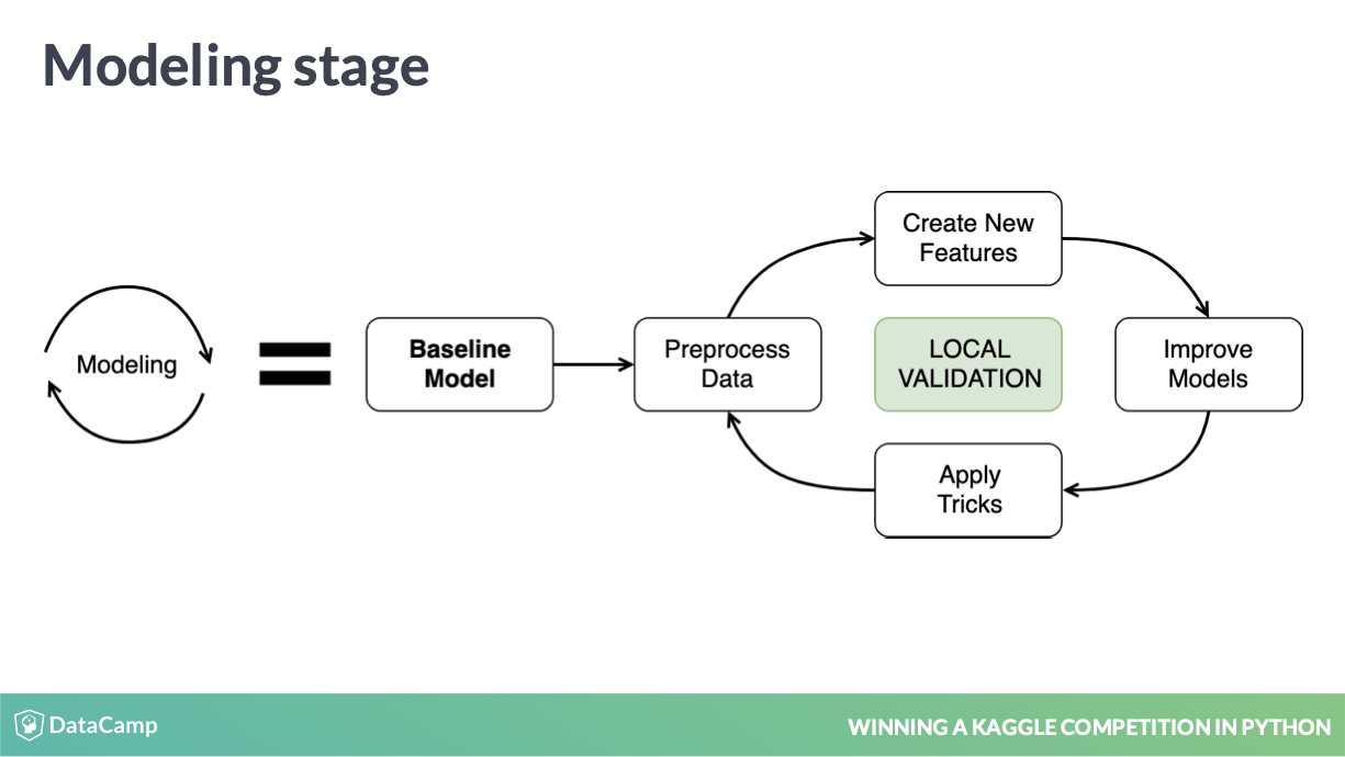
workflow

如图，最重要的是快速训练 baseline，跑通整个 workflow，其中每次快速迭代，都是靠可信的 local validation 进行的，因此

快速训练 baseline
可信的 local validation

是关键。

baseline model 就是为了去验证整个 workflow 是否可信的。为了避免歧义，我们应该是用 holdout set 来作为测试集的代名词。

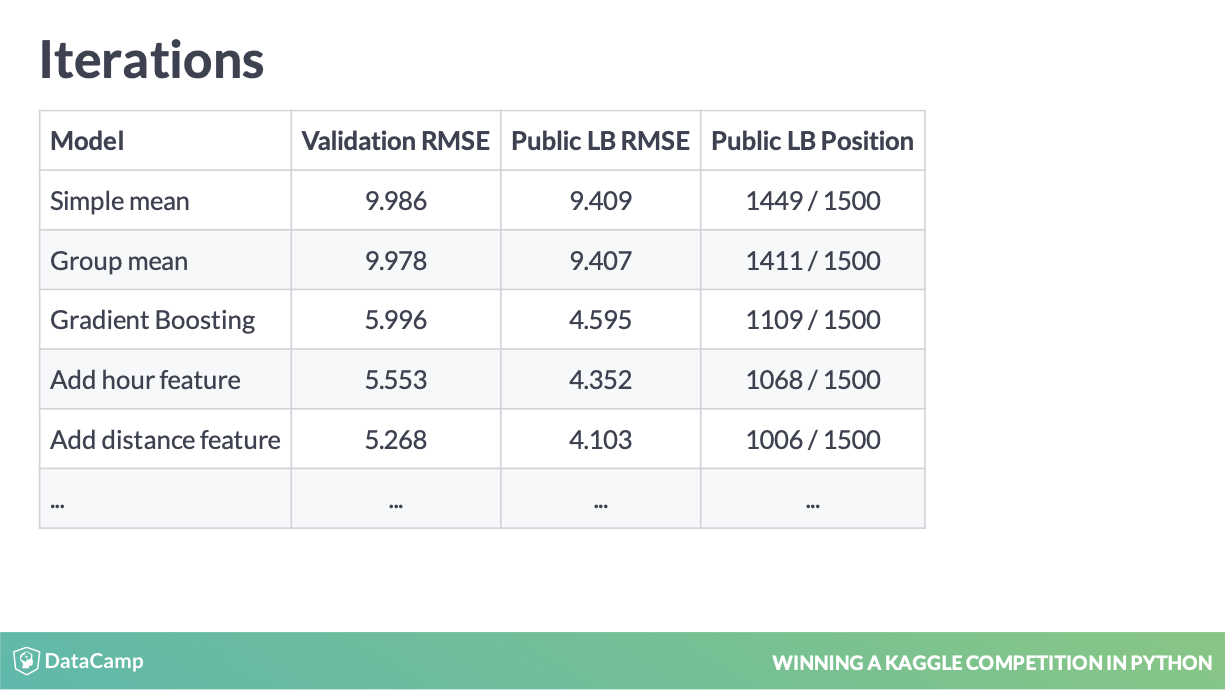
就是说 baseline model 可以用

naive mean，
naive cate variable mean，
xgboost

验证 workflow 中 local validation 和 leaderboard 之间是不是正相关，否则 local validation 不可信。

3 baseline model

3.1 mean baseline

import numpy as np
from sklearn.metrics import mean_squared_error
from math import sqrt

# Calculate average fare_amount on the validation_train data
naive_prediction = np.mean(validation_train.fare_amount)

# Assign naive prediction to all the holdout observations
validation_test['pred'] = naive_prediction

# Measure the local RMSE
rmse = sqrt(mean_squared_error(validation_test['fare_amount'], validation_test['pred']))
print('Validation RMSE for Baseline I model: {:.3f}'.format(rmse))

3.2 grouping baseline

test['fare_amount'] = test.hour.map(hour_groups)

这个地方的.map 非常有工程思想。

# Get pickup hour from the pickup_datetime column
train['hour'] = train['pickup_datetime'].dt.hour
test['hour'] = test['pickup_datetime'].dt.hour

# Calculate average fare_amount by pickup hour 
hour_groups = train.groupby(['hour']).fare_amount.mean()

# Make predicitons on the test set
test['fare_amount'] = test.hour.map(hour_groups)

# Write predictions
test[['id','fare_amount']].to_csv('hour_mean_sub.csv', index=False)

Also, remember to replicate all the results for the validation set as it was done in the previous exercise. (Babakhin 2019)

为了后期 stacking。注意这些模型都是为了测试 workflow 的，所以不要太上心效果，先把流程跑通。

3.3 random forest baseline

from sklearn.ensemble import RandomForestRegressor

# Select only numeric features
features = ['pickup_longitude', 'pickup_latitude', 'dropoff_longitude',
            'dropoff_latitude', 'passenger_count', 'hour']

# Train a Random Forest model
rf = RandomForestRegressor()
rf.fit(train[features], train.fare_amount)

# Make predictions on the test data
test['fare_amount'] = rf.predict(test[features])

# Write predictions
test[['id','fare_amount']].to_csv('rf_sub.csv', index=False)

So, now you know how to build fast and simple baseline models to validate your initial pipeline. (Babakhin 2019)

这很重要，模型要快速做出来。

4 Local Validation

You will be able to select the correct local validation scheme and to avoid overfitting. (Babakhin 2019)

本地验证方法是为了制造一个类似于 LeaderBoard 的验证集，以在线下查看模型的更新是否有提升，因为提交成绩有限，每次提升不可能都进行线上提交。

local validation 验证方式

这样我们观测 local validation 和 board 是不是同向变量，以此来判断 local validation 是否可靠。

4.1 Public and Private and Overfitting

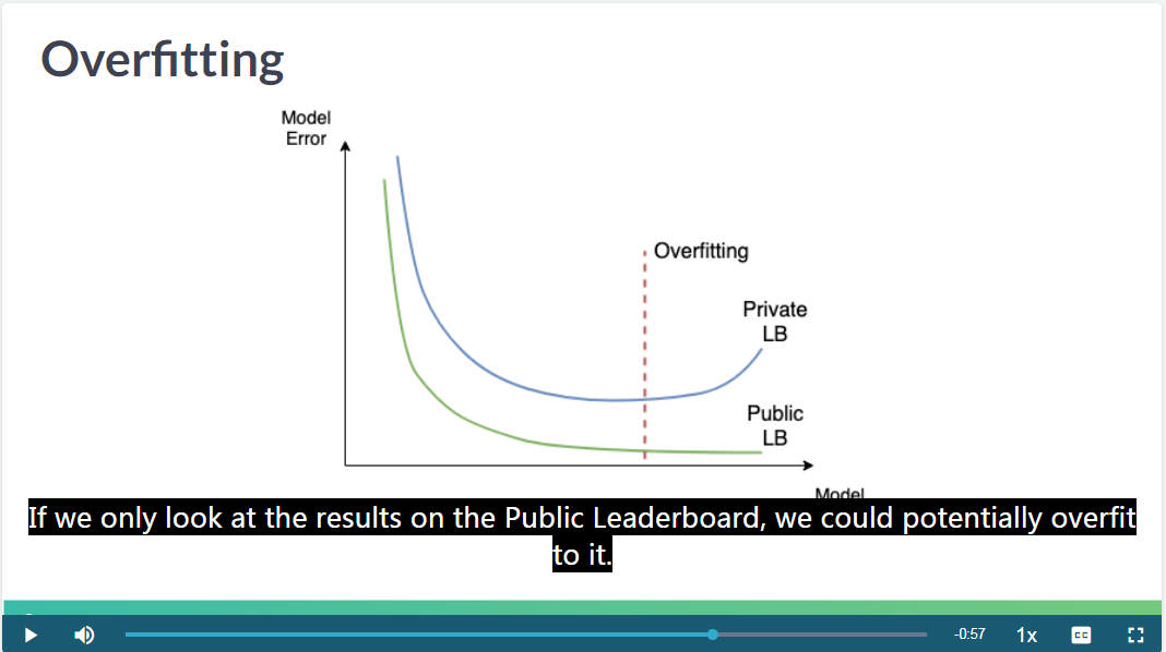
公开榜和私有榜过拟合

过于追求 public leaderboard 也是过拟合的一种表现。

You will learn the difference between Public and Private test splits, and how to prevent overfitting. (Babakhin 2019)

公开榜和私有榜之间的数据虽然不公开，但是也会存在过拟合情况。因此常看到私有榜靠前的人，在公开榜上排名并不靠前，这是因为公开榜靠前的成绩都是过拟合的。

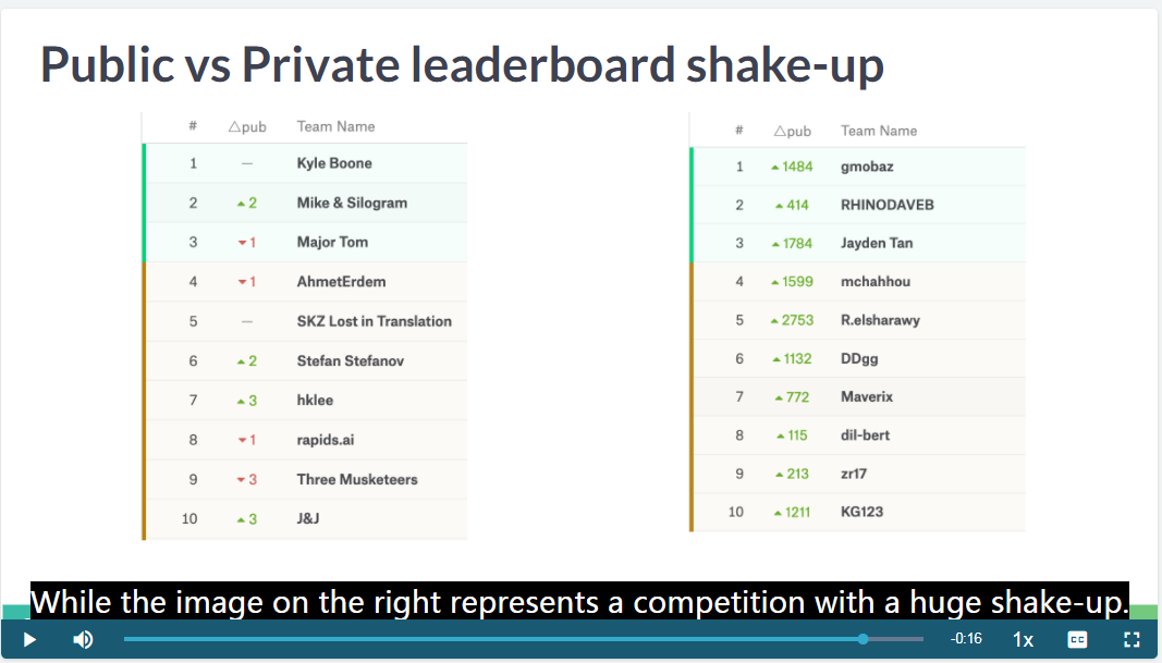
shake-up 的发生场景

public leaderboard shake-up 很严重，侧面反映了 public leaderboard 的失真。

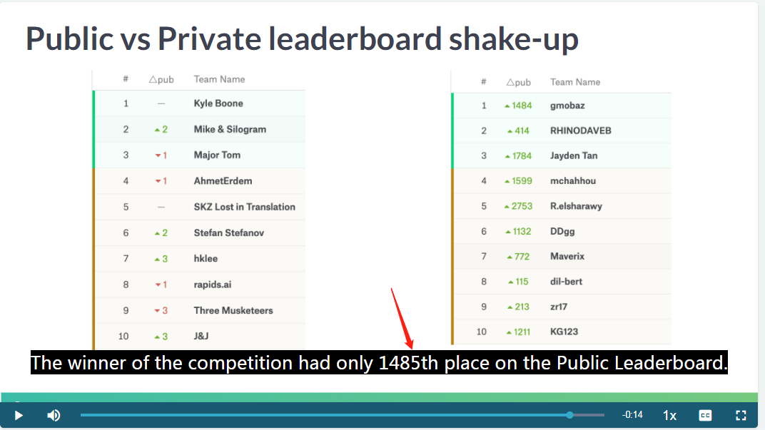
private leaderboard 实际上在公开榜排在1400多名。

因此 Babakhin (2019) 对过拟合的见解是很独到的。

4.2 Holdout set

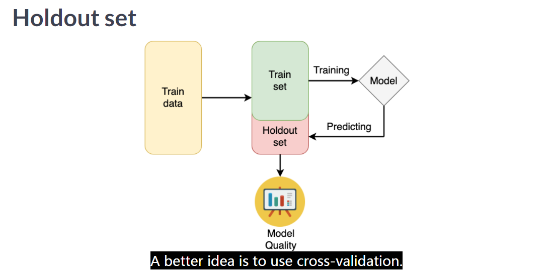
image

用 holdout set 是可以阻止一些过拟合，但是也是会过拟合的。为什么？因为始终只用同一个 extracted 的数据集进行 validate 就有问题，因此才引入 cross-validation。这种情况类似于 Public LeaderBoard 过拟合现象 4.1 。

4.3 案例

以比赛 Google Cloud & NCAA® ML Competition 2020-NCAAM | Kaggle 为例，public board 的验证集已经在数据集中公布，所以是一个很好的构建 local validation 并进行验证的机会。

path_list = []
local_valid = []
dir_path = "../submission/"
for path in os.listdir(dir_path):
    submission_path = os.path.join(dir_path,path)
    test_submission = pd.read_csv(submission_path)
    test_submission_loc_valid = test_submission[answer['Pred']!=0.5]
    
    logloss_value = log_loss(answer_loc_valid['Pred'],test_submission_loc_valid['Pred'])
    
    path_list.append(path)
    local_valid.append(logloss_value)

D:\install\miniconda\lib\site-packages\ipykernel_launcher.py:3: RuntimeWarning: divide by zero encountered in log
  This is separate from the ipykernel package so we can avoid doing imports until

local_valid_df = pd.DataFrame(zip(path_list,local_valid),columns=['fileName','local_valid'])

local_valid_df.sort_values('fileName', ascending=[False])

	fileName	local_valid
7	submission-20200306-180624.csv	0.113736
6	submission-20200306-172122.csv	0.118307
5	submission-20200306-170449.csv	0.118860
4	submission-20200306-164630.csv	0.122715
3	submission-20200306-162932.csv	0.128428
2	submission-20200306-160828.csv	0.405731
1	submission-20200306-154807.csv	0.152427
0	submission-20200301-195712.csv	inf

fileName	date	description	status	publicScore	privateScore
submission-20200306-180624.csv	2020-03-06 10:13:33	change n fold to 100	complete	0.11217	None
submission-20200306-172122.csv	2020-03-06 09:36:21	change n fold to 50	complete	0.11676	None
submission-20200306-170449.csv	2020-03-06 09:05:40	change n fold to 40	complete	0.11711	None
submission-20200306-164630.csv	2020-03-06 08:50:29	change n fold to 30	complete	0.12090	None
submission-20200306-162932.csv	2020-03-06 08:31:06	change n fold to 20.	complete	0.12624	None
submission-20200306-160828.csv	2020-03-06 08:09:55	add id embedding.	complete	0.41290	None
submission-20200306-154807.csv	2020-03-06 07:49:37	baseline with ratan123/march-madness-2020-ncaam-simple-lightgbm-on-kfold	complete	0.14907	None
submission-20200301-195712.csv	2020-03-06 07:21:23	baseline with original hyperparameters	complete	1.54431	None

基本是都是同增同减。为什么不是完全一致？根据 LogLoss 的定义来看，参考章节 12.8.3.1 参考潘越，因为考虑到预测值为0和1的情况，所以线上会加一个很小的数来防止出现inf，所以我们线下测和在线测会有一点点不一样。

5 基本树模型结构

我们会基本回避 LR (太依赖特征工程)，神经网络 (太依赖算力)，树模型是比较好的平衡。

6 K-Fold

注意 XGBoost 是加了 k_fold 这个参数的，所以已经使用了 cross-validation 思想了。

6.1 k-fold

# Import KFold
from sklearn.model_selection import KFold

# Create a KFold object
kf = KFold(n_splits=3, shuffle=True, random_state=123)

# Loop through each split
fold = 0
for train_index, test_index in kf.split(train):
    # Obtain training and testing folds
    cv_train, cv_test = train.iloc[train_index], train.iloc[test_index]
    print('Fold: {}'.format(fold))
    print('CV train shape: {}'.format(cv_train.shape))
    print('Medium interest listings in CV train: {}\n'.format(sum(cv_train.interest_level == 'medium')))
    fold += 1

这个代码在切分训练集和测试集时，非常有 sense。

<script.py> output:
    Fold: 0
    CV train shape: (666, 9)
    Medium interest listings in CV train: 175
    
    Fold: 1
    CV train shape: (667, 9)
    Medium interest listings in CV train: 165
    
    Fold: 2
    CV train shape: (667, 9)
    Medium interest listings in CV train: 162

6.2 Stratified K-fold

So, we see that the number of observations in each fold is almost uniform. It means that we’ve just split the train data into 3 equal folds. However, if we look at the number of medium-interest listings, it’s varying from 162 to 175 from one fold to another. To make them uniform among the folds, let’s use Stratified K-fold! (Babakhin 2019)

实际上这样分的话，对于我们 target 还是有点误差，因此可以分层抽样去管理。

# Import StratifiedKFold
from sklearn.model_selection import StratifiedKFold

# Create a StratifiedKFold object
str_kf = StratifiedKFold(n_splits=3, shuffle=True, random_state=123)

# Loop through each split
fold = 0
for train_index, test_index in str_kf.split(train, train.interest_level):
    # Obtain training and testing folds
    cv_train, cv_test = train.iloc[train_index], train.iloc[test_index]
    print('Fold: {}'.format(fold))
    print('CV train shape: {}'.format(cv_train.shape))
    print('Medium interest listings in CV train: {}\n'.format(sum(cv_train.interest_level == 'medium')))
    fold += 1

这是分层抽样的结果。

<script.py> output:
    Fold: 0
    CV train shape: (666, 9)
    Medium interest listings in CV train: 167
    
    Fold: 1
    CV train shape: (666, 9)
    Medium interest listings in CV train: 167
    
    Fold: 2
    CV train shape: (668, 9)
    Medium interest listings in CV train: 168

一般来说，对于分类问题，都会喜欢分层抽样超过一半的k-fold。

Great! Now you see that both size and target distribution are the same among the folds. The general rule is to prefer Stratified K-Fold over usual K-Fold in any classification problem. (Babakhin 2019)

6.3 time series k-fold

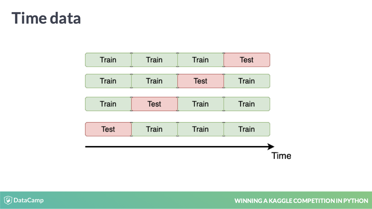
失效的CV方式

会产生 Data Leakage 12.9。

正确的处理方式

一般来说使用场景上，可以参考比赛 Store Item Demand Forecasting Challenge | Kaggle

You will work with another Kaggle competition called “Store Item Demand Forecasting Challenge”. In this competition, you are given 5 years of store-item sales data, and asked to predict 3 months of sales for 50 different items in 10 different stores. (Babakhin 2019)

可以明显发现，这里的 test 组受到时间的影响强烈，因此在 cv 上需要做好 time seris 的处理，这样也可以避免了时间序列模型（普遍认为 ARIMA 等模型的预测效果有限）。

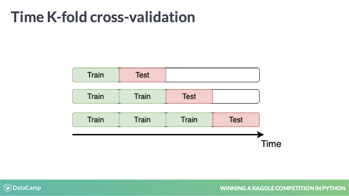
Remember the “Store Item Demand Forecasting Challenge” where you are given store-item sales data and have to predict future sales?

It’s a competition with time-series data. So, time K-fold cross-validation should be applied. Your goal is to create this cross-validation strategy and make sure that it works as expected. (Babakhin 2019)

# Create TimeSeriesSplit object
time_kfold = TimeSeriesSplit(n_splits=3)

# Sort train data by date
train = train.sort_values("date")

# Iterate through each split
fold = 0
for train_index, test_index in time_kfold.split(train):
    cv_train, cv_test = train.iloc[train_index], train.iloc[test_index]
    
    print('Fold :', fold)
    print('Train date range: from {} to {}'.format(cv_train.date.min(), cv_train.date.max()))
    print('Test date range: from {} to {}\n'.format(cv_test.date.min(), cv_test.date.max()))
    fold += 1

这是非常简洁的 Python 代码。

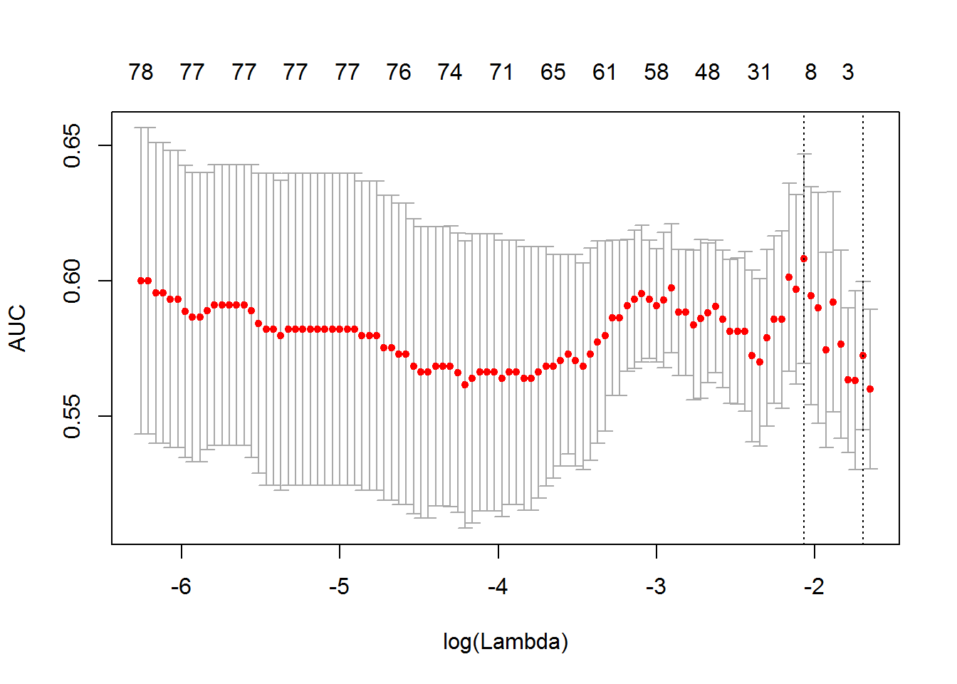
6.4 ts-k-fold 评价指标表现异常

以下是一个营销场景下的二分类模型，也是使用了时间进行分割训练和验证集。

xgb_eval_log <- read_rds("../data/xgb_evaluation_log.rds")

xgb_eval_log %>% head() %>% knitr::kable("markdown")

iter	train_auc	validation_auc
1	0.686319	0.701624
2	0.698362	0.714407
3	0.698475	0.711080
4	0.701082	0.715856
5	0.701537	0.715868
6	0.704749	0.715861

从模型第一次迭代开始，train 和 valid 的 auc 就差异出现，并且 valid 更高。

xgb_eval_log %>% 
    gather(key,value,-iter) %>% 
    ggplot() +
    geom_line(aes(x=iter,y=value,col=key))

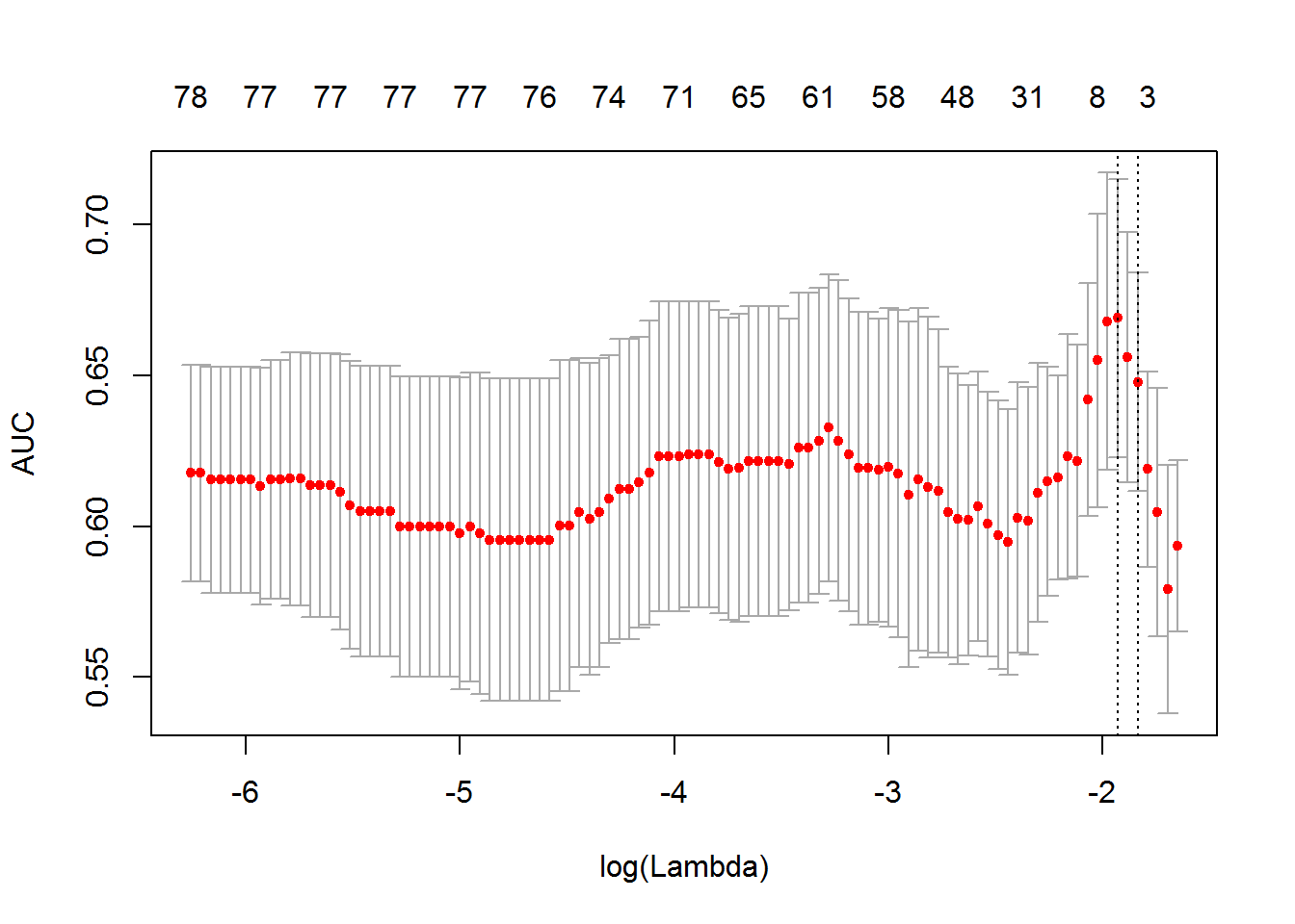
为了验证这种情况，我们可以再看下 KS

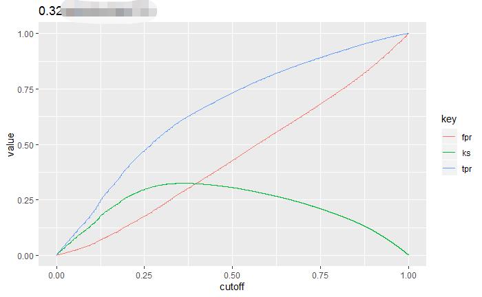
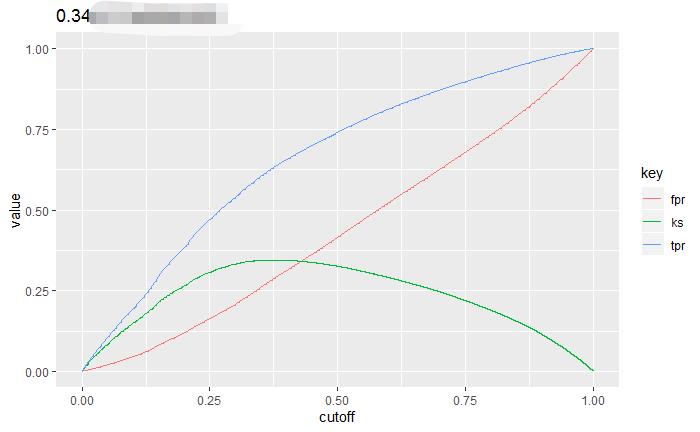
knitr::include_graphics("figure/train_ks.jpg")
knitr::include_graphics("figure/test_ks.jpg")

Figure 6.1: 训练集和验证集KS比较

我们来分析下为什么。首先按照 ts-k-fold 的情况。 train 和 valid 是不随机的。

我们选择某时间点之前为训练集之后为测试集，因此训练的模型，本身就可以偶然的在测试集上表现更高，比如

在 valid 中，与 y 正相关的变量更大
在 valid 中，与 y 负相关的变量更小

我们的算法只会限定

valid 的评价指标不要变差，也就是 early stopping 的目的
我们用过拟合的参数是为了让 valid 不要比 train 差，而不是控制 valid 不要比 train 好

因此当 valid 评价指标表现更高时，超参数是不限制的。

但是当随机的情况时，

在 valid 中，与 y 正相关的变量应该和 train 的差不多大
在 valid 中，与 y 负相关的变量应该和 train 的差不多小

因此正常情况下，train 和 valid 的评价指标应该一样，但是训练的模型是更容易拟合训练集的(因为梯度下降的loss来自训练集)，所以train通常会表现更好。

6.5 自定义 internal 函数

def get_fold_mse(train, kf):
    mse_scores = []
    
    for train_index, test_index in kf.split(train):
        fold_train, fold_test = train.loc[train_index], train.loc[test_index]

        # Fit the data and make predictions
        # Create a Random Forest object
        rf = RandomForestRegressor(n_estimators=10, random_state=123)

        # Train a model
        rf.fit(X=fold_train[['store', 'item']], y=fold_train['sales'])

        # Get predictions for the test set
        pred = rf.predict(fold_test[['store', 'item']])
    
        fold_score = round(mean_squared_error(fold_test['sales'], pred), 5)
        mse_scores.append(fold_score)
        
    return mse_scores

这些函数我都可以整合。

6.6 CV 整体效果指标

from sklearn.model_selection import TimeSeriesSplit
import numpy as np

# Sort train data by date
train = train.sort_values('date')

# Initialize 3-fold time cross-validation
kf = TimeSeriesSplit(n_splits=3)

# Get MSE scores for each cross-validation split
mse_scores = get_fold_mse(train, kf)

print('Mean validation MSE: {:.5f}'.format(np.mean(mse_scores)))
print('MSE by fold: {}'.format(mse_scores))
print('Overall validation MSE: {:.5f}'.format(np.mean(mse_scores) + np.std(mse_scores)))

np.mean(mse_scores) 就是 MSE 的等价物，并且 np.std(mse_scores) 也有统计意义，反正差异大，也不好。 Babakhin (2019) 对 overall model performance 的见解挺不错的。这样的思路也见于 R 包 glmnet，使用函数cv.glmnet后反馈的对象中也包含 cvm 和 cvsd

6.7 保存 Fold Id

fold_id = kf.split(df)
import pickle as pkl
for (idx,i) in enumerate(fold_id):
    print(idx)
    file_name = '../model/fold_id_{}.pkl'.format(idx)
    print('{} saved.'.format(file_name))
    with open(file_name, 'wb') as f:
        pkl.dump(i, f)

0 ../model/fold_id_0.pkl saved. 1 ../model/fold_id_1.pkl saved. 2 ../model/fold_id_2.pkl saved. 3 ../model/fold_id_3.pkl saved. 4 ../model/fold_id_4.pkl saved. 5 ../model/fold_id_5.pkl saved. 6 ../model/fold_id_6.pkl saved. 7 ../model/fold_id_7.pkl saved. 8 ../model/fold_id_8.pkl saved. 9 ../model/fold_id_9.pkl saved. 10 ../model/fold_id_10.pkl saved. 11 ../model/fold_id_11.pkl saved. 12 ../model/fold_id_12.pkl saved. 13 ../model/fold_id_13.pkl saved. 14 ../model/fold_id_14.pkl saved. 15 ../model/fold_id_15.pkl saved. 16 ../model/fold_id_16.pkl saved. 17 ../model/fold_id_17.pkl saved. 18 ../model/fold_id_18.pkl saved. 19 ../model/fold_id_19.pkl saved.

$ du -sh model/fold_id* | clip
18M model/fold_id_0.pkl
18M model/fold_id_1.pkl
18M model/fold_id_10.pkl
18M model/fold_id_11.pkl
18M model/fold_id_12.pkl
18M model/fold_id_13.pkl
18M model/fold_id_14.pkl
18M model/fold_id_15.pkl
18M model/fold_id_16.pkl
18M model/fold_id_17.pkl
18M model/fold_id_18.pkl
18M model/fold_id_19.pkl
18M model/fold_id_2.pkl
18M model/fold_id_3.pkl
18M model/fold_id_4.pkl
18M model/fold_id_5.pkl
18M model/fold_id_6.pkl
18M model/fold_id_7.pkl
18M model/fold_id_8.pkl
18M model/fold_id_9.pkl

一般都比较大，fold id 文件，所以建议 ignore 的。

7 特征工程

7.1 Arithmetical features

这就是我们说的用业务知识合成的变量。

a new feature representing the area of the garden. It is a difference between the total area of the property (“LotArea”) and the first-floor area (“1stFlrSF”).

Create a new feature representing the total number of bathrooms in the house. It is a sum of full bathrooms (“FullBath”) and half bathrooms (“HalfBath”).

# Look at the initial RMSE
print('RMSE before feature engineering:', get_kfold_rmse(train))

# Add total area of the house
train['TotalArea'] = train['TotalBsmtSF'] + train['1stFlrSF'] + train['2ndFlrSF']
print('RMSE with total area:', get_kfold_rmse(train))

# Add garden area of the property
train['GardenArea'] = train['LotArea'] - train['1stFlrSF']
print('RMSE with garden area:', get_kfold_rmse(train))

# Add total number of bathrooms
train['TotalBath'] = train['FullBath'] + train['HalfBath']
print('RMSE with number of bathrooms:', get_kfold_rmse(train))

模型封装好后，就可以这样比较字段好坏 6.5 。

<script.py> output:
    RMSE before feature engineering: 36029.39
    RMSE with total area: 35073.2
    RMSE with garden area: 34413.55
    RMSE with number of bathrooms: 34506.78

不是每次特征工程都是好的，应该模块分开，这类本身可以在 SQL 层面完成。

7.2 Date features

# Concatenate train and test together
taxi = pd.concat([train, test])

# Convert pickup date to datetime object
taxi['pickup_datetime'] = pd.to_datetime(taxi['pickup_datetime'])

# Create day of week feature
taxi['day_of_week'] = taxi['pickup_datetime'].dt.dayofweek

# Create hour feature
taxi['hour'] = taxi['pickup_datetime'].dt.hour

# Split back into train and test
new_train = taxi[taxi.id.isin(train.id)]
new_test = taxi[test.id.isin(test.id)]

这种分解 id 的方法我觉得非常可取。并且到 stacking 上时，也可以用这种方式 predict 所有的 yhat。

但是，我觉得 R tibbletime 包做了完美的集成方案。

8 Feature Encoding

8.1 (Integer)Label Encoding

这是一种常见方式已经在 sklearn 内置，广泛应用和到生产。

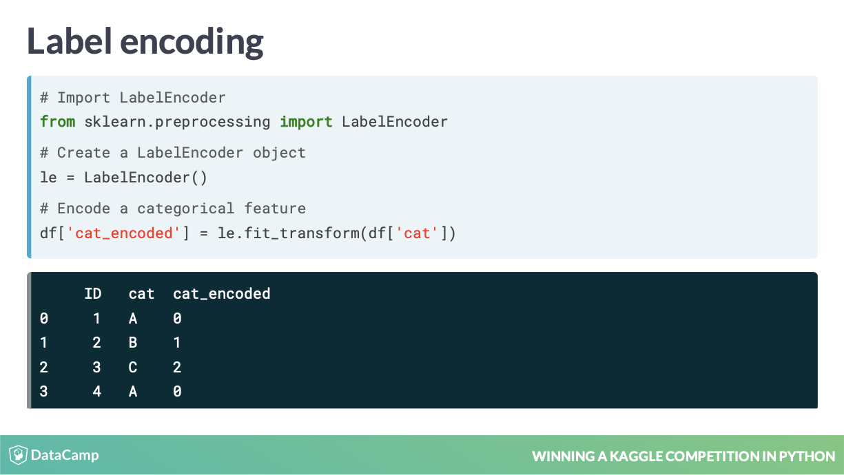
参考代码

# Concatenate train and test together
houses = pd.concat([train, test])

# Label encoder
from sklearn.preprocessing import LabelEncoder
le = LabelEncoder()

# Create new features
houses['RoofStyle_enc'] = le.fit_transform(houses['RoofStyle'])
houses['CentralAir_enc'] = le.fit_transform(houses['CentralAir'])

# Look at new features
print(houses[['RoofStyle', 'RoofStyle_enc', 'CentralAir', 'CentralAir_enc']].head())

<script.py> output:
      RoofStyle  RoofStyle_enc CentralAir  CentralAir_enc
    0     Gable              1          Y               1
    1     Gable              1          Y               1
    2     Gable              1          Y               1
    3     Gable              1          Y               1
    4     Gable              1          Y               1

8.2 One-Hot encoding

# Concatenate train and test together
houses = pd.concat([train, test])

# Label encode binary 'CentralAir' feature
from sklearn.preprocessing import LabelEncoder
le = LabelEncoder()
houses['CentralAir_enc'] = le.fit_transform(houses['CentralAir'])

# Create One-Hot encoded features
ohe = pd.get_dummies(houses['RoofStyle'], prefix='RoofStyle')

# Concatenate OHE features to houses
houses = pd.concat([houses, ohe], axis=1)

# Look at OHE features
print(houses[[col for col in houses.columns if 'RoofStyle' in col]].head(3))

<script.py> output:
      RoofStyle  RoofStyle_Flat  RoofStyle_Gable  RoofStyle_Gambrel  RoofStyle_Hip  RoofStyle_Mansard  RoofStyle_Shed
    0     Gable               0                1                  0              0                  0               0
    1     Gable               0                1                  0              0                  0               0
    2     Gable               0                1                  0              0                  0               0

最后一步操作在工程上会非常稳定，不会因为新的 test 集而导致产生 unknown factors。

8.3 Mean target encoding

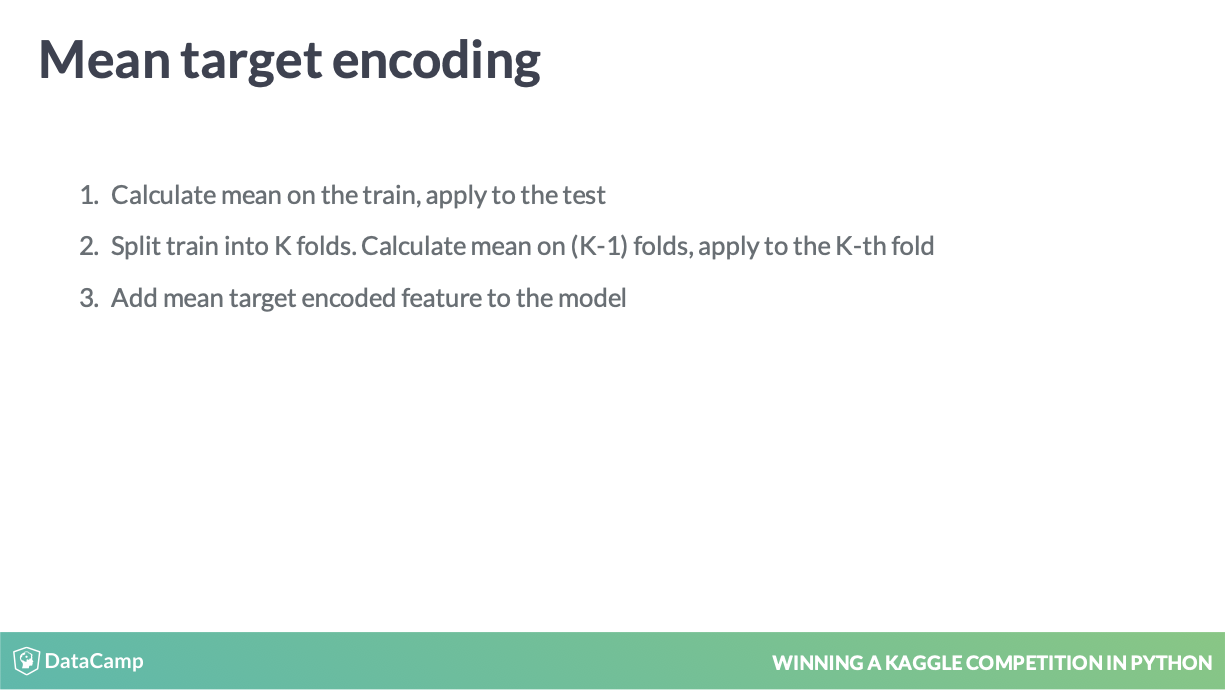
模块化变量

关于 global mean 等的实现方式，这个还需要在思考思考。就是为了加入 smoothing 但是其实 k-fold 等 idea 看代码会更好的理解。

train_statistics = (category_sum + global_mean * alpha) / (category_size + alpha)

这个地方类似于 Laplace 变换。

test_feature = test[categorical].map(train_statistics).fillna(global_mean)

缺失值使用 global mean 也非常符合逻辑。

def test_mean_target_encoding(train, test, target, categorical, alpha=5):
    # Calculate global mean on the train data
    global_mean = train[target].mean()
    
    # Group by the categorical feature and calculate its properties
    train_groups = train.groupby(categorical)
    category_sum = train_groups[target].sum()
    category_size = train_groups.size()
    
    # Calculate smoothed mean target statistics
    train_statistics = (category_sum + global_mean * alpha) / (category_size + alpha)
    
    # Apply statistics to the test data and fill new categories
    test_feature = test[categorical].map(train_statistics).fillna(global_mean)
    return test_feature.values

引入 train_feature = pd.Series(index=train.index) 是为了最后方便用 cv 值填补。

train_feature.iloc[test_index] = cv_test_feature

def train_mean_target_encoding(train, target, categorical, alpha=5):
    # Create 5-fold stratified cross-validation
    skf = StratifiedKFold(n_splits=5, random_state=123, shuffle=True)
    train_feature = pd.Series(index=train.index)
    
    # For each folds split
    for train_index, test_index in skf.split(train, train[target]):
        cv_train, cv_test = train.iloc[train_index], train.iloc[test_index]
      
        # Calculate out-of-fold statistics and apply to cv_test
        cv_test_feature = test_mean_target_encoding(cv_train, cv_test, target, categorical, alpha)
        
        # Save new feature for this particular fold
        train_feature.iloc[test_index] = cv_test_feature       
    return train_feature.values

这是做了 k-fold 管理了。

def mean_target_encoding(train, test, target, categorical, alpha=5):
  
    # Get test feature
    test_feature = test_mean_target_encoding(train, test, target, categorical, alpha)
    
    # Get train feature
    train_feature = train_mean_target_encoding(train, target, categorical, alpha)
    
    # Return new features to add to the model
    return train_feature, test_feature

最后是完整的函数。

# Create 5-fold cross-validation
kf = KFold(n_splits=5, random_state=123, shuffle=True)

# For each folds split
for train_index, test_index in kf.split(bryant_shots):
    cv_train, cv_test = bryant_shots.iloc[train_index], bryant_shots.iloc[test_index]
    
    # Create mean target encoded feature
    cv_train['game_id_enc'], cv_test['game_id_enc'] = mean_target_encoding(train=cv_train,
                                                                           test=cv_test,
                                                                           target="shot_made_flag",
                                                                           categorical="game_id",
                                                                           alpha=5)
    # Look at the encoding
    print(cv_train[['game_id', 'shot_made_flag', 'game_id_enc']].sample(n=1))

这是从应用角度上看到的。

更值得说的是

cv_train['game_id_enc'], cv_test['game_id_enc'] = mean_target_encoding(train=cv_train,
                                                                           test=cv_test,
                                                                           target="shot_made_flag",
                                                                           categorical="game_id",
                                                                           alpha=5)

我从函数层面就可以完成这种简洁的赋值方式了。

<script.py> output:
           game_id  shot_made_flag  game_id_enc
    7106  20500532             0.0     0.439732
           game_id  shot_made_flag  game_id_enc
    5084  20301100             0.0     0.524644
           game_id  shot_made_flag  game_id_enc
    6687  20500228             0.0     0.328546
           game_id  shot_made_flag  game_id_enc
    5046  20301075             0.0     0.296946
           game_id  shot_made_flag  game_id_enc
    4662  20300515             1.0     0.513995

mean target encoding 还可以应用到其他非二分类的模型中。

For binary classification usually mean target encoding is used For regression mean could be changed to median, quartiles, etc. For multi-class classification with N classes we create N features with target mean for each category in one vs. all fashion (Babakhin 2019)

# Create mean target encoded feature
train['RoofStyle_enc'], test['RoofStyle_enc'] = mean_target_encoding(train=train,
                                                                     test=test,
                                                                     target='SalePrice',
                                                                     categorical='RoofStyle',
                                                                     alpha=10)
# Look at the encoding
print(test[['RoofStyle', 'RoofStyle_enc']].drop_duplicates())

对于回归问题的应用。

you’ve encoded categorical feature in such a manner that there is now a correlation between category values and target variable.

这是处理 integer encoding 更好的方式。

8.4 缺失值

不是很有意思，目前 XGBoost 和 LightGBM 已经可以自动处理。 -999 在 linear model 里面不好，但是在 tree model 里面很好，这里背书了。

# Read dataframe
twosigma = pd.read_csv('twosigma_train.csv')

# Find the number of missing values in each column
print(twosigma.isnull().sum())

# Look at the columns with missing values
print(twosigma[['building_id','price']].head())

# Import SimpleImputer
from sklearn.impute import SimpleImputer

# Create constant imputer
constant_imputer = SimpleImputer(strategy="constant", fill_value="MISSING")

# building_id imputation
rental_listings[['building_id']] = constant_imputer.fit_transform(rental_listings[['building_id']])

# Import SimpleImputer
from sklearn.impute import SimpleImputer

# Create mean imputer
mean_imputer = SimpleImputer(strategy="mean")

# Price imputation
rental_listings[['price']] = mean_imputer.fit_transform(rental_listings[['price']])

9 Grid search

# Possible max depth values
max_depth_grid = [3, 6, 9, 12, 15]
results = {}

# For each value in the grid
for max_depth_candidate in max_depth_grid:
    # Specify parameters for the model
    params = {'max_depth': max_depth_candidate}

    # Calculate validation score for a particular hyperparameter
    validation_score = get_cv_score(train, params)

    # Save the results for each max depth value
    results[max_depth_candidate] = validation_score   
print(results)

for 循环是非常容易理解的工程代码方式。

<script.py> output:
    {3: 6.50509, 6: 6.52138, 9: 6.64181, 12: 6.8819, 15: 6.99156}

Nice! We have a validation score for each value in the grid. The optimal max depth value is located somewhere between 3 and 6. The next step could be to use a smaller grid, for example [3, 4, 5, 6] and repeat the same process. Moving from larger to smaller grids allows us to find the most optimal values. Keep going to try optimizing two hyperparameters simultaneously! (Babakhin 2019)

这种缩小范围的 grid search 思想很常见。这种迭代过程的代码，写得很好，值得我后期在 R 上也优化。

Apply the product() function from the itertools package to the hyperparameter grids. It returns all possible combinations for these two grids.

类似于 R 中的 hyper.grid 函数。

from itertools import product

# Hyperparameter grids
max_depth_grid = [3,5,7]
subsample_grid = [0.8,0.9,1.0]
results = {}

# For each couple in the grid
for max_depth_candidate, subsample_candidate in product(max_depth_grid, subsample_grid):
    params = {'max_depth': max_depth_candidate,
              'subsample': subsample_candidate}
    validation_score = get_cv_score(train, params)
    # Save the results for each couple
    results[(max_depth_candidate, subsample_candidate)] = validation_score   
print(results)

Great! You can see that tuning multiple hyperparameters simultaneously achieves better results. In the previous exercise, tuning only the max_depth parameter gave the best RMSE of $6.50. With max_depth equal to 7 and subsample equal to 0.8, the best RMSE is now $6.16. However, do not spend too much time on the hyperparameter tuning at the beginning of the competition! Another approach that almost always improves your solution is model ensembling. Go on for it! (Babakhin 2019)

不建议在比赛初期，大多数数据挖掘方法没有实现时，就开始超参数调整。

10 model ensembling

理解 stacking 和 blending，这些方法是在比赛中成功得出的经验。

10.1 blending

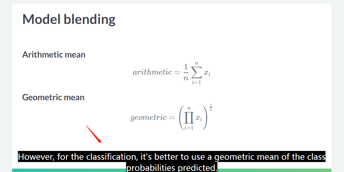
分类模型的话，比较建议使用 geometric mean。

from sklearn.ensemble import GradientBoostingRegressor, RandomForestRegressor

# Train a Gradient Boosting model
gb = GradientBoostingRegressor().fit(train[features], train['fare_amount'])

# Train a Random Forest model
rf = RandomForestRegressor().fit(train[features], train['fare_amount'])

# Make predictions on the test data
test['gb_pred'] = gb.predict(test[features])
test['rf_pred'] = rf.predict(test[features])

# Find mean of model predictions
test['blend'] = (test['gb_pred']+test['rf_pred']) / 2
print(test[['gb_pred', 'rf_pred', 'blend']].head(3))

<script.py> output:
        gb_pred  rf_pred     blend
    0  9.661374     9.00  9.330687
    1  9.304288     8.45  8.877144
    2  5.795140     5.11  5.452570

10.2 stacking

Split train data into two parts

Train multiple models on Part 1

Make predictions on Part 2

Make predictions on the test data

Train a new model on Part 2 using predictions as features

Make predictions on the test data using the 2nd level model

data => train + hold-out
train => p1 + p2
p1 训练 1st-level 模型，并且给出 p2 和 hold-out 组上的预测，之后 p2 预测值用于训练，hold-out 预测值用于 2nd-level 模型预测
p2 训练 2nd-level 模型，也叫做 meta-model，在 hold-out 上进行预测

from sklearn.model_selection import train_test_split
from sklearn.ensemble import GradientBoostingRegressor, RandomForestRegressor

# Split train data into two parts
part_1, part_2 = train_test_split(train, test_size=0.5, random_state=123)

# Train a Gradient Boosting model on Part 1
gb = GradientBoostingRegressor().fit(part_1[features], part_1.fare_amount)

# Train a Random Forest model on Part 1
rf = RandomForestRegressor().fit(part_1[features], part_1.fare_amount)

# Make predictions on the Part 2 data
part_2['gb_pred'] = gb.predict(part_2[features])
part_2['rf_pred'] = rf.predict(part_2[features])

# Make predictions on the test data
test['gb_pred'] = gb.predict(test[features])
test['rf_pred'] = rf.predict(test[features])

from sklearn.linear_model import LinearRegression

# Create linear regression model without the intercept
lr = LinearRegression(fit_intercept=False)

# Train 2nd level model in the part_2 data
lr.fit(part_2[['gb_pred', 'rf_pred']], part_2.fare_amount)

# Make stacking predictions on the test data
test['stacking'] = lr.predict(test[['gb_pred', 'rf_pred']])

# Look at the model coefficients
print(lr.coef_)

<script.py> output:
    [0.72504358 0.27647395]

Usually, the 2nd level model is some simple model like Linear or Logistic Regressions. Also, note that you were not using intercept in the Linear Regression just to combine pure model predictions. Looking at the coefficients, it’s clear that 2nd level model has more trust in the Gradient Boosting: 0.7 versus 0.3 for the Random Forest model. (Babakhin 2019)

这是一些业界的思路，不要用截距。

11 保存中间过程

11.1 output 构成

Save folds to the disk
Save model runs
Save model predictions to the disk
Save performance results

从可重复性研究角度，以上对象都需要保存，也方便做 history stacking。

11.2 不保存 foldid 的后果

library(magrittr)

load("rawdata_v1.rdata")
y <- rawdata$items %>% as.factor
x <- rawdata[,-1] %>% as.matrix()
# 变量脱敏
x %<>%
    `names<-`(1:ncol(x))

library(glmnet)

set.seed(1)
cvfit1 <- cv.glmnet(x,
                    y,
                    family = "binomial",
                    type.measure = "auc",
                    nfolds = 5,
                    keep = TRUE)

set.seed(2)
cvfit2 <- cv.glmnet(x,
                    y,
                    family = "binomial",
                    type.measure = "auc",
                    nfolds = 5,
                    keep = TRUE)

coef(cvfit1) %>% dim

## [1] 25473     1

coef(cvfit2) %>% dim

## [1] 25473     1

# lambda.min: value of lambda that gives minimum cvm.
mean(coef(cvfit1) == coef(cvfit2))

## [1] 0.999843

# 不用 seed 下，预测 beta 一致。

coef(cvfit1)[,1] %>% head

##        (Intercept) ENSG00000000003.14  ENSG00000000005.6 ENSG00000000419.12 
##         -0.2989249          0.0000000          0.0000000          0.0000000 
## ENSG00000000457.14 ENSG00000000460.17 
##          0.0000000          0.0000000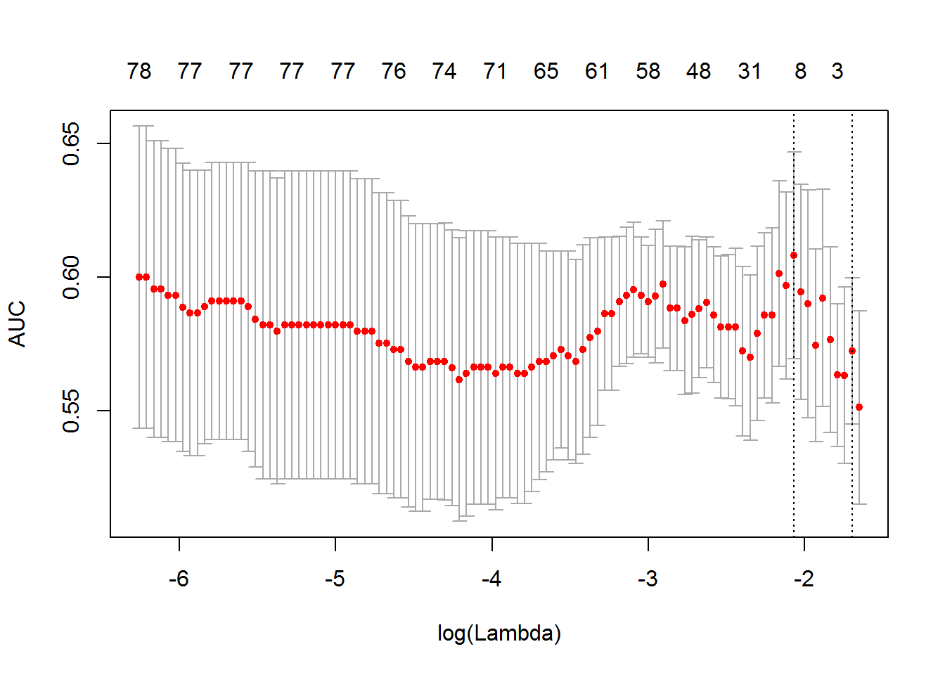

# 你可以验证下

plot(cvfit1)

plot(cvfit2)

cvfit1$lambda.min

## [1] 0.1262239

cvfit2$lambda.min

## [1] 0.1451269

不一样是因为交叉验证在不同随机状态下 fold 不一样的。

nrow(rawdata)

## [1] 96

cvfit1$foldid #这是 fold 的切分方式

##  [1] 3 4 1 4 2 3 4 2 4 1 5 1 4 4 2 3 4 2 5 3 4 3 5 5 2 3 5 3 1 1 5 2 5 5 1 1 3 5
## [39] 2 2 1 4 2 5 2 5 3 2 3 1 4 1 2 3 5 5 3 1 2 1 3 4 3 1 3 1 4 4 3 4 2 1 1 4 1 2
## [77] 2 4 5 2 1 4 5 5 1 3 2 3 1 3 5 2 4 5 5 4

mean(cvfit1$foldid ==cvfit2$foldid) # 可以发现放在 fold 设置是一样的情况的话，只有20%

## [1] 0.21875

查看 help 文档，这里不要在随机状态下设置 nfolds 固定 foldid 查看情况。

set.seed(1)
cvfit1.1 <- cv.glmnet(x,
                    y,
                    family = "binomial",
                    type.measure = "auc",
                    foldid = cvfit1$foldid,
                    keep = TRUE)

set.seed(2)
cvfit2.1 <- cv.glmnet(x,
                    y,
                    family = "binomial",
                    type.measure = "auc",
                    foldid = cvfit1$foldid,
                    keep = TRUE)

cvfit1.1$lambda.min

## [1] 0.1262239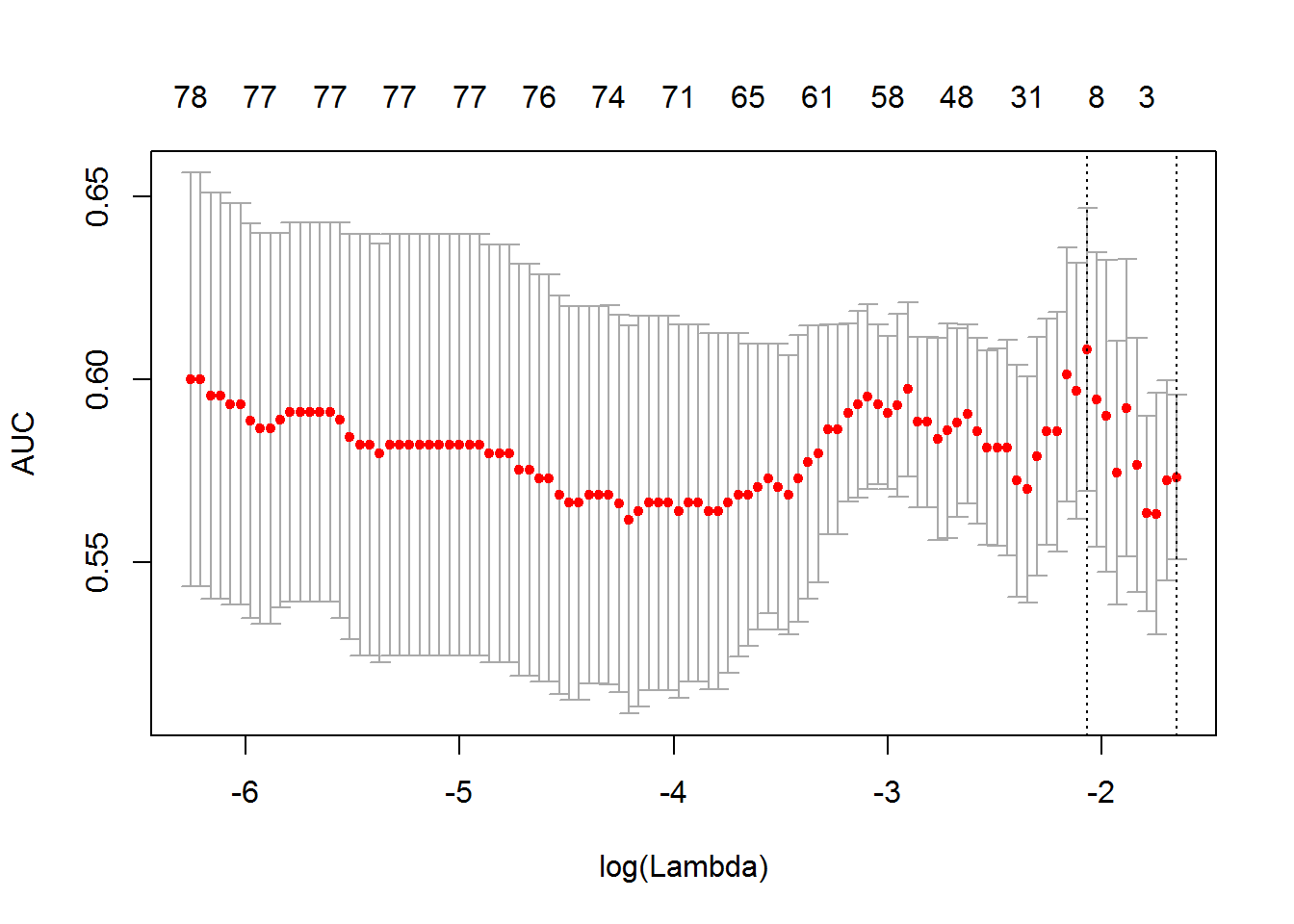

cvfit1.1$lambda.min == cvfit2.1$lambda.min # 现在查看就一致了

## [1] TRUE

plot(cvfit1.1)

plot(cvfit2.1)

总结来说，seed 不同，cv 的分组肯定不同，导致的各种指标如 mse、lambda 肯定要不同，否则就失去了随机的意义。

我们一般在打 Kaggle 比赛的时候，会比较不同模型之间的效果，我们会把 k-fold 的 foldid 保存(Babakhin 2019, Chapter 4)。因为 foldid 的选择受到了 set.seed() 影响，两个不是独立的，在模型比较时会出现两个扰动项

不同foldid下导致评价指标不同
模型之间效率的差异导致评价指标不同，这才是我们想要的

为了把第一种扰动项剔除，我们会把 foldid 给固定。

12 Playground Competition

我们会对以上进行的数据挖掘的方法进行比赛上的验证，Playground 是不算难的，但是成绩靠前，需要进行较长时间的特征工程或者神经网络学习(GPU) 12.10，我们目前只讨论前者，以下比赛可以进行测试，加入对应的队伍。

12.1 Store Item Demand Forecasting Challenge

Store Item Demand Forecasting Challenge | Kaggle Jiaxiang Li

This is a Kernels-only competition, all your submissions will be made from a Kaggle Kernel. Please see the screenshots on how to make a submission from Kernels.

因此比赛需要在 Kaggle Notebook 上完成，不能在本地训练。

12.1.1 local validation

Kaggle Notebook https://www.kaggle.com/lijiaxiang/local-validation

filename public_score local_rmse
baseline_v1.0.0.csv 48.91844 28.772
baseline_v1.1.0.csv 45.16562 26.868
baseline_v1.2.0.csv 28.34696 15.856 
stacking_v1.0.0.csv 28.42869 15.860

这是 local validation 测试的结果。

Submissions are evaluated on SMAPE between forecasts and actual values. We define SMAPE = 0 when the actual and predicted values are both 0. https://www.kaggle.com/c/demand-forecasting-kernels-only/overview/evaluation (Babakhin 2019)

所以两者是正相关的，说明 local validation 有效。

12.1.2 k-fold

Kaggle Notebook https://www.kaggle.com/lijiaxiang/kfold-type

12.1.3 stacking

Kaggle Notebook https://www.kaggle.com/lijiaxiang/stacking

print(lr.coef_)
[0.00243761 0.99905634]

没有体现出效果。也只能说 GradientBoostingRegressor 效果不好，

print(lr.coef_)
[0.00250759 0.99854456]

没有体现出效果。也只能说 XGBoost 效果不好，

12.2 New York City Taxi Fare Prediction

New York City Taxi Fare Prediction | Kaggle Jiaxiang Li

数据很大，不好下载。train.csv (5.31 GB) 数据量太大不好弄，学习小样本进行训练。

For faster performance, you will work with a subsample consisting of 1,000 observations. (Babakhin 2019)

对啊，对于大的数据，我们为了展示的目的，可以这么处理。

12.2.1 local validation

Kaggle Notebook https://www.kaggle.com/lijiaxiang/local-validation-new-york-city-taxi-fare-pred 参考 https://www.kaggle.com/breemen/nyc-taxi-fare-data-exploration/ 进行 input 策略。

12.3 House Prices

House Prices: Advanced Regression Techniques | Kaggle 夕阳红

这个比赛变量较多，适合做特征工程。

12.3.1 local validation

Kaggle Notebook https://www.kaggle.com/lijiaxiang/local-validation-house-prices

附录

12.4 使用 Kaggle API 下载数据

参考 https://github.com/Kaggle/kaggle-api


$ kaggle kernels pull shubh24/pagerank-on-quora-a-basic-implementation
Source code downloaded to D:\work\imp_rmd\pagerank-on-quora-a-basic-implementation.ipynb


$ mkdir pagerank
pagerank/                                       pagerank-on-quora-a-basic-implementation.ipynb


$ mkdir pagerank
pagerank/                                       pagerank-on-quora-a-basic-implementation.ipynb


$ mv pagerank-on-quora-a-basic-implementation.ipynb pagerank


$ kaggle competitions download -c quora-question-pairs
Downloading test.csv.zip to D:\work\imp_rmd
  1%|▎                                                              | 1.00M/173M [00:00<02:42, 1.11MB/s]
  1%|▋                                                              | 2.00M/173M [00:01<02:24, 1.24MB/s]
  2%|█                                                              | 3.00M/173M [00:02<02:12, 1.35MB/s]
  2%|█▍                                                             | 4.00M/173M [00:02<02:05, 1.41MB/s
  3%|█▊                                                             | 5.00M/173M [00:03<01:54, 1.54MB/s
  3%|██▏                                                            | 6.00M/173M [00:03<01:43, 1.70MB/
  4%|██▌                                                            | 7.00M/173M [00:04<01:35, 1.82MB/
  5%|██▉                                                            | 8.00M/173M [00:04<01:30, 1.91MB/
  5%|███▎                                                           | 9.00M/173M [00:05<01:32, 1.86MB
  6%|███▋                                                           | 10.0M/173M [00:06<01:35, 1.80MB
  6%|███▉                                                           | 11.0M/173M [00:06<01:33, 1.82MB
  7%|████▎                                                          | 12.0M/173M [00:07<01:44, 1.61M
  7%|████▋                                                          | 13.0M/173M [00:08<01:48, 1.55M
  8%|█████                                                          | 14.0M/173M [00:08<01:43, 1.61M
  9%|█████▍                                                         | 15.0M/173M [00:09<01:41, 1.63
  9%|█████▊                                                         | 16.0M/173M [00:09<01:39, 1.66
 10%|██████▏                                                        | 17.0M/173M [00:10<01:41, 1.6
 10%|██████▌                                                        | 18.0M/173M [00:11<01:40, 1.6
 11%|██████▉                                                        | 19.0M/173M [00:12<01:42, 1.5
 12%|███████▎                                                       | 20.0M/173M [00:12<01:39, 1.
 12%|███████▋                                                       | 21.0M/173M [00:13<01:34, 1.
 13%|███████▉                                                       | 22.0M/173M [00:13<01:29, 1.
 13%|████████▎                                                      | 23.0M/173M [00:14<01:26, 1
 14%|████████▋                                                      | 24.0M/173M [00:14<01:21, 1
 14%|█████████                                                      | 25.0M/173M [00:15<01:25, 1
 15%|█████████▍                                                     | 26.0M/173M [00:16<01:34,
 16%|█████████▊                                                     | 27.0M/173M [00:16<01:41,
 16%|██████████▏                                                    | 28.0M/173M [00:17<01:53,
 17%|██████████▌                                                    | 29.0M/173M [00:18<02:00,
 17%|██████████▉                                                    | 30.0M/173M [00:19<01:59,
 18%|███████████▎                                                   | 31.0M/173M [00:20<01:47
 18%|███████████▋                                                   | 32.0M/173M [00:20<01:35
 19%|███████████▉                                                   | 33.0M/173M [00:21<01:26
 20%|████████████▎                                                  | 34.0M/173M [00:22<01:3
 20%|████████████▋                                                  | 35.0M/173M [00:22<01:4
 21%|█████████████                                                  | 36.0M/173M [00:24<01:5
 21%|█████████████▍                                                 | 37.0M/173M [00:25<02:
 22%|█████████████▊                                                 | 38.0M/173M [00:25<01:
 22%|██████████████▏                                                | 39.0M/173M [00:26<01
 23%|██████████████▌                                                | 40.0M/173M [00:26<01
 24%|██████████████▉                                                | 41.0M/173M [00:27<01
 24%|███████████████▎                                               | 42.0M/173M [00:28<0
 25%|███████████████▌                                               | 43.0M/173M [00:29<0
 25%|███████████████▉                                               | 44.0M/173M [00:30<0
 26%|████████████████▎                                              | 45.0M/173M [00:31<
 27%|████████████████▋                                              | 46.0M/173M [00:32<
 27%|█████████████████                                              | 47.0M/173M [00:33<
 28%|█████████████████▍                                             | 48.0M/173M [00:33
 28%|█████████████████▊                                             | 49.0M/173M [00:34
 29%|██████████████████▏                                            | 50.0M/173M [00:3
 29%|██████████████████▌                                            | 51.0M/173M [00:3
 30%|██████████████████▉                                            | 52.0M/173M [00:3
 31%|███████████████████▎                                           | 53.0M/173M [00:
 31%|███████████████████▌                                           | 54.0M/173M [00:
 32%|███████████████████▉                                           | 55.0M/173M [00:
 32%|████████████████████▎                                          | 56.0M/173M [00
 33%|████████████████████▋                                          | 57.0M/173M [00
 33%|█████████████████████                                          | 58.0M/173M [00
 34%|█████████████████████▍                                         | 59.0M/173M [0
 35%|█████████████████████▊                                         | 60.0M/173M [0
 35%|██████████████████████▏                                        | 61.0M/173M [
 36%|██████████████████████▌                                        | 62.0M/173M [
 36%|██████████████████████▉                                        | 63.0M/173M [
 37%|███████████████████████▎                                       | 64.0M/173M
 37%|███████████████████████▌                                       | 65.0M/173M
 38%|███████████████████████▉                                       | 66.0M/173M
 39%|████████████████████████▎                                      | 67.0M/173M
 39%|████████████████████████▋                                      | 68.0M/173M
 40%|█████████████████████████                                      | 69.0M/173M
 40%|█████████████████████████▍                                     | 70.0M/173
 41%|█████████████████████████▊                                     | 71.0M/173
 42%|██████████████████████████▏                                    | 72.0M/17
 42%|██████████████████████████▌                                    | 73.0M/17
 43%|██████████████████████████▉                                    | 74.0M/17
 43%|███████████████████████████▏                                   | 75.0M/1
 44%|███████████████████████████▌                                   | 76.0M/1
 44%|███████████████████████████▉                                   | 77.0M/1
 45%|████████████████████████████▎                                  | 78.0M/
 46%|████████████████████████████▋                                  | 79.0M/
 46%|█████████████████████████████                                  | 80.0M/
 47%|█████████████████████████████▍                                 | 81.0M
 47%|█████████████████████████████▊                                 | 82.0M
 48%|██████████████████████████████▏                                | 83.0
 48%|██████████████████████████████▌                                | 84.0
 49%|██████████████████████████████▉                                | 85.0
 50%|███████████████████████████████▏                               | 86.
 50%|███████████████████████████████▌                               | 87.
 51%|███████████████████████████████▉                               | 88.
 51%|████████████████████████████████▎                              | 89
 52%|████████████████████████████████▋                              | 90
 52%|█████████████████████████████████                              | 91
 53%|█████████████████████████████████▍                             | 9
 54%|█████████████████████████████████▊                             | 9
 54%|██████████████████████████████████▏                            |
 55%|██████████████████████████████████▌                            |
 55%|██████████████████████████████████▉                            |
 56%|███████████████████████████████████▏                           |
 57%|███████████████████████████████████▌                           |
 57%|███████████████████████████████████▉                           |
 58%|████████████████████████████████████▉
 58%|█████████████████████████████████████▎
 59%|█████████████████████████████████████▋
 59%|██████████████████████████████████████
 60%|██████████████████████████████████████▍
 61%|██████████████████████████████████████▊
 61%|███████████████████████████████████████
 62%|███████████████████████████████████████▍
 62%|███████████████████████████████████████▊
 63%|████████████████████████████████████████▏
 63%|████████████████████████████████████████▌
 64%|████████████████████████████████████████▉
 65%|█████████████████████████████████████████▎
 65%|█████████████████████████████████████████▋
 66%|██████████████████████████████████████████
 66%|██████████████████████████████████████████▍
 67%|██████████████████████████████████████████▊
 67%|███████████████████████████████████████████▏
 68%|███████████████████████████████████████████▌
 69%|███████████████████████████████████████████▉
 69%|████████████████████████████████████████████▎
 70%|████████████████████████████████████████████▋
 70%|█████████████████████████████████████████████
 71%|█████████████████████████████████████████████▍
 72%|█████████████████████████████████████████████▊
 72%|██████████████████████████████████████████████▏
 73%|██████████████████████████████████████████████▌
 73%|██████████████████████████████████████████████▊
 74%|███████████████████████████████████████████████▏
 74%|███████████████████████████████████████████████▌
 75%|███████████████████████████████████████████████▉
 76%|████████████████████████████████████████████████▎
 76%|████████████████████████████████████████████████▋
 77%|█████████████████████████████████████████████████
 77%|█████████████████████████████████████████████████▍
 78%|█████████████████████████████████████████████████▊
 78%|██████████████████████████████████████████████████
 79%|██████████████████████████████████████████████████
 80%|██████████████████████████████████████████████████
 80%|██████████████████████████████████████████████████
 81%|██████████████████████████████████████████████████
 81%|██████████████████████████████████████████████████
 82%|██████████████████████████████████████████████████
 82%|██████████████████████████████████████████████████
 83%|██████████████████████████████████████████████████
 84%|██████████████████████████████████████████████████
 84%|██████████████████████████████████████████████████
 85%|██████████████████████████████████████████████████
 85%|██████████████████████████████████████████████████
 86%|██████████████████████████████████████████████████
 87%|██████████████████████████████████████████████████
 87%|██████████████████████████████████████████████████
 88%|██████████████████████████████████████████████████
 88%|██████████████████████████████████████████████████
 89%|██████████████████████████████████████████████████
 89%|██████████████████████████████████████████████████
 90%|██████████████████████████████████████████████████
 91%|██████████████████████████████████████████████████
 91%|██████████████████████████████████████████████████
 92%|██████████████████████████████████████████████████
 92%|██████████████████████████████████████████████████
 93%|██████████████████████████████████████████████████
 93%|██████████████████████████████████████████████████
 94%|██████████████████████████████████████████████████
 95%|██████████████████████████████████████████████████
 95%|██████████████████████████████████████████████████
 96%|██████████████████████████████████████████████████
 96%|██████████████████████████████████████████████████
 97%|██████████████████████████████████████████████████
 97%|██████████████████████████████████████████████████
 98%|██████████████████████████████████████████████████
 99%|██████████████████████████████████████████████████
 99%|██████████████████████████████████████████████████
100%|██████████████████████████████████████████████████
100%|██████████████████████████████████████████████████
██████████████| 173M/173M [01:56<00:00, 1.25MB/s]

Downloading sample_submission.csv.zip to D:\work\imp_rmd
 20%|████████████▌                                                 | 1.00M/4.95M [00:00<00:0
 40%|█████████████████████████                                     | 2.00M/4.95M
 61%|█████████████████████████████████████▌
 81%|██████████████████████████████████████████████████
100%|██████████████████████████████████████████████████
████████████| 4.95M/4.95M [00:04<00:00, 1.21MB/s]

Downloading train.csv.zip to D:\work\imp_rmd
  5%|██▉                                                           | 1.00M/21.2M [00:00<00:14, 1.43MB/
  9%|█████▊                                                        | 2.00M/21.2M [00:01<00:13, 1.52
 14%|████████▊                                                     | 3.00M/21.2M [00:01<00:11, 1
 19%|███████████▋                                                  | 4.00M/21.2M [00:02<00:10
 24%|██████████████▋                                               | 5.00M/21.2M [00:03<00
 28%|█████████████████▌                                            | 6.00M/21.2M [00:03
 33%|████████████████████▍                                         | 7.00M/21.2M [00
 38%|███████████████████████▍                                      | 8.00M/21.2M
 43%|██████████████████████████▎                                   | 9.00M/21.
 47%|█████████████████████████████▎                                | 10.0M/
 52%|████████████████████████████████▏                             | 11.
 57%|███████████████████████████████████▏                          |
 61%|██████████████████████████████████████
 66%|████████████████████████████████████████▉
 71%|███████████████████████████████████████████▉
 76%|██████████████████████████████████████████████▊
 80%|█████████████████████████████████████████████████▊
 85%|██████████████████████████████████████████████████
 90%|██████████████████████████████████████████████████
 94%|██████████████████████████████████████████████████
 99%|██████████████████████████████████████████████████
100%|██████████████████████████████████████████████████
████████████| 21.2M/21.2M [00:14<00:00, 1.26MB/s]

参考 https://github.com/Kaggle/kaggle-api 下载数据。

kaggle datasets files wendykan/lending-club-loan-data
name                   size  creationDate         
---------------------  ----  -------------------  
database.sqlite         1GB  2019-03-18 18:43:12  
LCDataDictionary.xlsx  23KB  2019-03-18 18:43:12  
loan.csv                1GB  2019-03-18 18:43:12

kaggle datasets download wendykan/lending-club-loan-data -p input

12.5 使用 Kaggle API 传输成绩

$ kaggle competitions submit -c titanic -f demo_catboost.csv -m "catboost baseline model"
401 - Unauthorized

重新 Create API Token

一般也是无效的，因为这和科学上网的问题有关系，需要设置特定的VPN。

$ kaggle competitions submit -c google-cloud-ncaa-march-madness-2020-division-1-mens-tournament -f submission/submission-20200301-195712.csv -m "baseline with original hyperparameters"
  0%|                                                                      | 0.00/392k [00:00<?, ?B/s]2
020-03-01 20:17:08,214 WARNING Retrying (Retry(total=9, connect=None, read=None, redirect=None, status=
None)) after connection broken by 'NewConnectionError('<urllib3.connection.VerifiedHTTPSConnection obje
ct at 0x00000000040889E8>: Failed to establish a new connection: [WinError 10060] 由于连接方在一段时间

12.6 如果API在两台设备上用 Kaggle API

Warning: Your Kaggle API key is readable by other users on this system! To fix this, you can run ‘chmod 600 /root/.kaggle/kaggle.json’

chmod 600 /root/.kaggle/kaggle.json

12.7 Kaggle benefits

Get practical experience on the real-world data

Develop portfolio projects

Meet a great Data Science community

Try a new domain or model type

Keep up-to-date with the best performing methods

其实 Stacking 这些方法我都是在 Kaggle 先接触到，毕竟业界是要比学界对方法的更新更快。

12.8 常用公式

12.8.1 RMSLE

\[R M S L E=\sqrt{\frac{1}{N} \sum_{i=1}^{N}\left(\log \left(y_{i}+1\right)-\log \left(\hat{y}_{i}+1\right)\right)^{2}}\]

12.8.2 RMSE

import numpy as np

# Import MSE from sklearn
from sklearn.metrics import mean_squared_error

# Define your own MSE function
def own_mse(y_true, y_pred):
    # Find squared differences
    squares = np.power(y_true - y_pred, 2)
    # Find mean over all observations
    err = np.mean(squares)
    return err

print('Sklearn MSE: {:.5f}. '.format(mean_squared_error(y_regression_true, y_regression_pred)))
print('Your MSE: {:.5f}. '.format(own_mse(y_regression_true, y_regression_pred)))

12.8.3 LogLoss

\[\text {LogLoss}=-\frac{1}{N} \sum_{i=1}^{N}\left(y_{i} \log p_{i}+\left(1-y_{i}\right) \log \left(1-p_{i}\right)\right)\]

import numpy as np

# Import log_loss from sklearn
from sklearn.metrics import log_loss

# Define your own LogLoss function
def own_logloss(y_true, prob_pred):
    # Find loss for each observation
    terms = y_true * np.log(prob_pred) + (1 - y_true) * np.log(1 - prob_pred)
    # Find mean over all observations
    err = np.mean(terms) 
    return -err

print('Sklearn LogLoss: {:.5f}'.format(log_loss(y_classification_true, y_classification_pred)))
print('Your LogLoss: {:.5f}'.format(own_logloss(y_classification_true, y_classification_pred)))

12.8.3.1 使用 logloss 的注意事项

预测值不能为0或者1

import numpy as np
true_y_0 = 0.5;pred_h_0=0.000
-np.mean(true_y_0*np.log(pred_h_0)+(1-true_y_0)*np.log(1-pred_h_0))

## inf
## 
## D:\install\MINICO~1\python.exe:1: RuntimeWarning: divide by zero encountered in log

np.log(pred_h_0),np.log(0)

## (-inf, -inf)

true_y_0 = 0.5;pred_h_0=1.000
-np.mean(true_y_0*np.log(pred_h_0)+(1-true_y_0)*np.log(1-pred_h_0))

## inf

np.log(pred_h_0),np.log(0)

## (0.0, -inf)

logloss 预测值不能为0，不然输出是 Inf。

但是这在打比赛的时候难以发现，但是会给一个极差的成绩。

fileName	date	description	status	publicScore	privateScore
submission-20200306-180624.csv	2020-03-06 10:13:33	change n fold to 100	error	0.11217	None
submission-20200306-172122.csv	2020-03-06 09:36:21	change n fold to 50	error	0.11676	None
submission-20200306-170449.csv	2020-03-06 09:05:40	change n fold to 40	error	0.11711	None
submission-20200306-164630.csv	2020-03-06 08:50:29	change n fold to 30	error	0.12090	None
submission-20200306-162932.csv	2020-03-06 08:31:06	change n fold to 20.	error	0.12624	None
submission-20200306-160828.csv	2020-03-06 08:09:55	add id embedding.	complete	0.41290	None
submission-20200306-154807.csv	2020-03-06 07:49:37	baseline with ratan123/march-madness-2020-ncaam-simple-lightgbm-on-kfold	error	0.14907	None
submission-20200301-195712.csv	2020-03-06 07:21:23	baseline with original hyperparameters	complete	1.54431	None

注意成绩submission-20200301-195712.csv就是极差的。

skim_output <-
    read.csv("../../ncaa-march-madness-2020/submission/submission-20200301-195712.csv") %>%
    skimr::skim()

print(skim_output)

## Skim summary statistics
##  n obs: 11390 
##  n variables: 2 
## 
## -- Variable type:factor --------------------------------------------------------------------------------------
##  variable missing complete     n n_unique                     top_counts
##        ID       0    11390 11390    11390 201: 1, 201: 1, 201: 1, 201: 1
##  ordered
##    FALSE
## 
## -- Variable type:numeric -------------------------------------------------------------------------------------
##  variable missing complete     n mean  sd p0   p25   p50  p75 p100     hist
##      Pred       0    11390 11390 0.26 0.4  0 0.025 0.025 0.49    1 ▇▁▁▁▁▁▁▂

查看到预测值中存在0和1。这需要替换。

import numpy as np
np.clip(1,0.001,0.999)

## 0.999

12.8.4 距离函数

def haversine_distance(train):
    
    data = [train]
    lat1, long1, lat2, long2 = 'pickup_latitude', 'pickup_longitude', 'dropoff_latitude', 'dropoff_longitude'
    
    for i in data:
        R = 6371  #radius of earth in kilometers
        #R = 3959 #radius of earth in miles
        phi1 = np.radians(i[lat1])
        phi2 = np.radians(i[lat2])
    
        delta_phi = np.radians(i[lat2]-i[lat1])
        delta_lambda = np.radians(i[long2]-i[long1])
    
        #a = sin²((φB - φA)/2) + cos φA . cos φB . sin²((λB - λA)/2)
        a = np.sin(delta_phi / 2.0) ** 2 + np.cos(phi1) * np.cos(phi2) * np.sin(delta_lambda / 2.0) ** 2
    
        #c = 2 * atan2( √a, √(1−a) )
        c = 2 * np.arctan2(np.sqrt(a), np.sqrt(1-a))
    
        #d = R*c
        d = (R * c) #in kilometers
        
    return d

# Calculate the ride distance
train['distance_km'] = haversine_distance(train)

# Draw a scatterplot
plt.scatter(train.fare_amount, train.distance_km, alpha=0.5)
plt.xlabel('Fare amount')
plt.ylabel('Distance, km')
plt.title('Fare amount based on the distance')

# Limit on the distance
plt.ylim(0, 50)
plt.show()

12.8.5 单变量图

画单变量图， y ~ x 的。

# Create hour feature
train['pickup_datetime'] = pd.to_datetime(train.pickup_datetime)
train['hour'] = train.pickup_datetime.dt.hour

# Find median fare_amount for each hour
hour_price = train.groupby('hour', as_index=False)['fare_amount'].median()

# Plot the line plot
plt.plot(hour_price.hour, hour_price.fare_amount, marker='o')
plt.xlabel('Hour of the day')
plt.ylabel('Fare amount')
plt.title('Fare amount based on day time')
plt.xticks(range(24))
plt.show()

这是一种查看变量简单的思路，方便和业务解释。

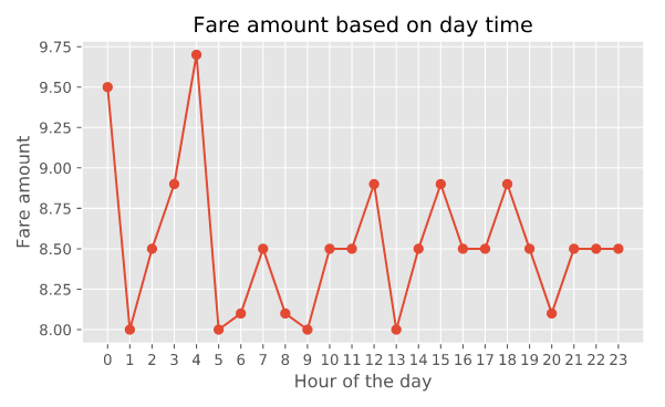
image

至少在这里，波动很厉害，差异很大，也不是 random，那么就是很好的用 tree 模型去搞的方式。

12.9 Data Leakage

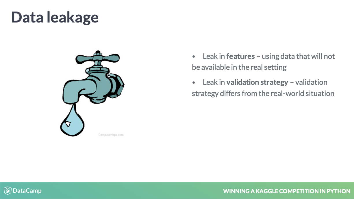
事后变量和失效的 CV 方法

第二种的情况发生在数据如股票等，严格受到时间影响，但是 CV 时，把靠后的样本预测靠前的样本了。

12.10 调参数和特征工程的差异

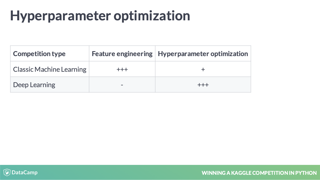
深度学习和经典机器学习的差异

深度学习才是调参数为重，机器学习模型主要还是在变量上！

12.11 完成证书

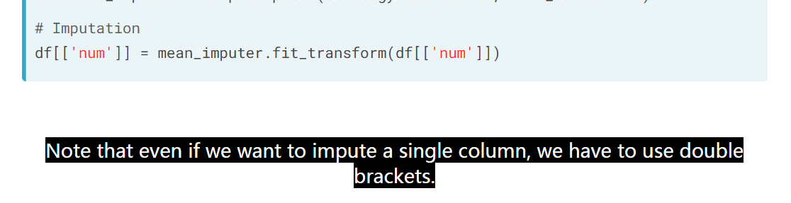
12.12 impute 变量用双括号

image

这个是 Python 的一个sense

12.13 打私人榜的建议

所以私人榜和 local validation 的记录都要保留。

参考文献

Babakhin, Yauhen. 2019. “Winning a Kaggle Competition in Python.” DataCamp. 2019. https://www.datacamp.com/courses/winning-a-kaggle-competition-in-python.

Kaggle 学习笔记

1 安排

2 模型训练思路

2.1 workflow

3 baseline model

3.1 mean baseline

3.2 grouping baseline

3.3 random forest baseline

4 Local Validation

4.1 Public and Private and Overfitting

4.2 Holdout set

4.3 案例

5 基本树模型结构

6 K-Fold

6.1 k-fold

6.2 Stratified K-fold

6.3 time series k-fold

6.4 ts-k-fold 评价指标表现异常

6.5 自定义 internal 函数

6.6 CV 整体效果指标

6.7 保存 Fold Id

7 特征工程

7.1 Arithmetical features

7.2 Date features

8 Feature Encoding

8.1 (Integer)Label Encoding

8.2 One-Hot encoding

8.3 Mean target encoding

8.4 缺失值

9 Grid search

10 model ensembling

10.1 blending

10.2 stacking

11 保存中间过程

11.1 output 构成

11.2 不保存 foldid 的后果

12 Playground Competition

12.1 Store Item Demand Forecasting Challenge

12.1.1 local validation

12.1.2 k-fold

12.1.3 stacking

12.2 New York City Taxi Fare Prediction

12.2.1 local validation

12.3 House Prices

12.3.1 local validation

附录

12.4 使用 Kaggle API 下载数据

12.5 使用 Kaggle API 传输成绩

12.6 如果API在两台设备上用 Kaggle API

12.7 Kaggle benefits

12.8 常用公式

12.8.1 RMSLE

12.8.2 RMSE

12.8.3 LogLoss

12.8.3.1 使用 logloss 的注意事项

12.8.4 距离函数

12.8.5 单变量图

12.9 Data Leakage

12.10 调参数和特征工程的差异

12.11 完成证书

12.12 impute 变量用双括号

12.13 打私人榜的建议

参考文献