使用 RMarkdown 的 child 参数，进行文档拼接。
这样拼接以后的笔记方便复习。
相关问题提交到 GitHub

1 kNN

1.1 kNN 概念

KNN算法又称k近邻分类 (k-nearest neighbor classification) 算法。它是根据不同特征值之间的距离来进行分类的一种简单的机器学习方法，它是一种简单但是懒惰的算法。他的训练数据都是有标签的数据。 blog

The full k-nearest neighbors algorithm works much in the way some of us ask for recommendations from our friends. First, we start with people whose taste we feel we share, and then we ask a bunch of them to recommend something to us. If many of them recommend the same thing, we deduce that we’ll like it as well. (Conway and White 2012)

这里朋友即说明了我朋友和我很近，那么他们喜欢的东西，我也喜欢，即使我没有历史记录。

Another approach would be to use the points nearest the point you’re trying to classify to make your guess. You could, for example, draw a circle around the point you’re looking at and then decide on a classification based on the points within that circle. Figure 10-3 shows just such an approach, which we’ll quickly call the “Grassroots Democracy” algorithm. (Conway and White 2012)

Xs 定义了空间上各点的距离。那么点的 \(\hat y\) 来源于周围 k 个临近点的 \(y\) 的投票。因此这是一个比较“民主”的投票 (Grassroots Democracy)。

include_graphics("https://user-images.githubusercontent.com/15884785/58630570-66de3780-8312-11e9-83f8-ff382ce3b0df.png")

Figure 1.1: 对于图中第二种情况，决策树和逻辑回归就很难完成了。

include_graphics("https://user-images.githubusercontent.com/15884785/58630581-7198cc80-8312-11e9-9557-fd260bc55e77.png")

Figure 1.2: 对于图中第二种情况，决策树和逻辑回归就很难完成了。

If all of your data points have their neighbors at roughly the same distance, this won’t be a problem. But if some points have many close neighbors while others have almost none, you’ll end up picking a circle that’s so big it extends well past the decision boundaries for some points. What can we do to work around this problem? The obvious solution is to avoid using a circle to define a point’s neighbors and instead look at the k-closest points. (Conway and White 2012)

不要用半径，而用最近的。因此这是 KMeans 和 KNN 的主要区别。

1.2 kNN 底层实现

df <- read.csv('../refs/example_data.csv')

df %>% dim

## [1] 100   3

df %>% head

X、Y就是特征变量，Label就是标签，进行 kNN 监督学习。

distance.matrix <- function(df) {
    distance <- matrix(rep(NA, nrow(df) ^ 2), nrow = nrow(df))
    for (i in 1:nrow(df)) {
        for (j in 1:nrow(df)) {
            distance[i, j] <-
                sqrt((df[i, 'X'] - df[j, 'X']) ^ 2 + (df[i, 'Y'] - df[j, 'Y']) ^ 2)
        }
    }
    return(distance)
}

source(here::here("R/k_nearest_neighbors.R"))

knn <- function(df, k = 5) {
    distance <- distance.matrix(df)
    predictions <- rep(NA, nrow(df))
    for (i in 1:nrow(df)) {
        indices <- k_nearest_neighbors(i, distance, k = k)
        predictions[i] <-
            ifelse(mean(df[indices, 'Label']) > 0.5, 1, 0)
    }
    return(predictions)
}

也就是说只要加载这样一个训练集，建立一个空间，每次预测集样本进行空间拟合就好了。

df %>% 
    mutate(pred = knn(df)) %>% 
    summarise(mean(Label != pred))

1.3 与LR效果比较

df <- read.csv('../refs/example_data.csv')

n <- nrow(df)
set.seed(1)
indices <- sort(sample(1:n, n * (1 / 2)))
training.x <- df[indices, 1:2]
test.x <- df[-indices, 1:2]
training.y <- df[indices, 3]
test.y <- df[-indices, 3]
predicted.y <-
    class::knn(training.x, test.x, training.y, k = 5) 
mean(predicted.y != test.y)

## [1] 0.14

logit.model <- glm(Label ~ X + Y, data = df[indices, ])
predictions <- as.numeric(predict(logit.model, newdata = df[-indices, ]) > 0)
mean(predictions != test.y)

## [1] 0.48

显然这个样本的 kNN 效果更好，我们来分析下样本。

df %>% 
    mutate(Label = as.factor(Label)) %>% 
    ggplot() +
    aes(X, Y, col = Label) +
    geom_point() +
    scale_color_manual(values = wesanderson::wes_palette("Royal1"))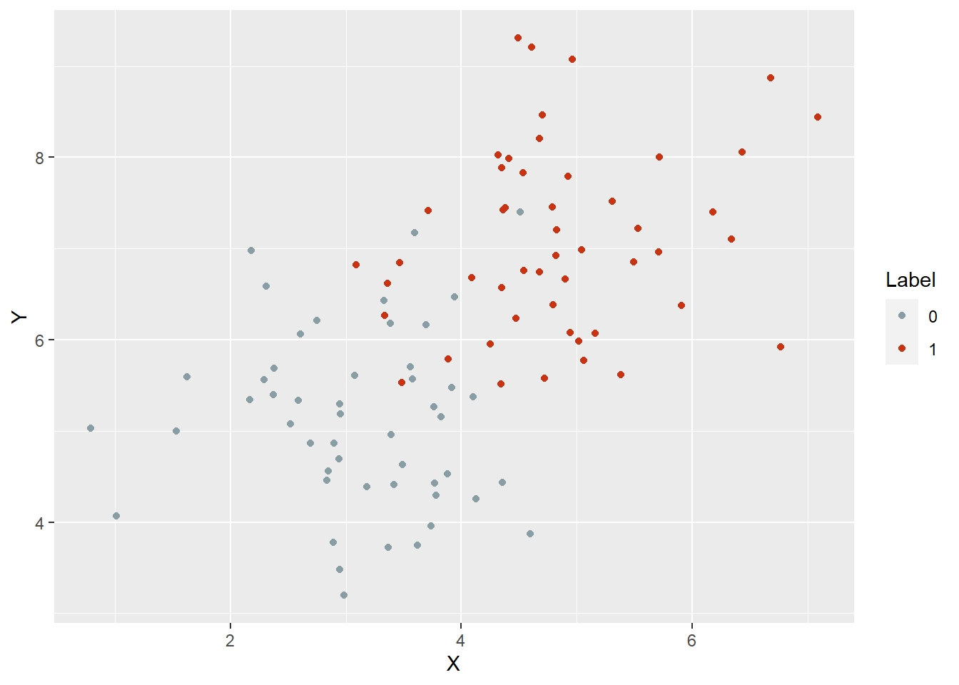

很明显，这样一个界限明显的样本，kNN 都比逻辑回归表现好，因此评分卡模型特征工程太重要了。

When your problem is far from being linear, kNN will work out of the box much better than other methods. [Conway2012Machine]

目前来看效果比逻辑回归好。

1.4 kNN 推荐系统

One way we could start to make recommendations is to find items that are similar to the items our users already like and then apply kNN, which we’ll call the item-based approach. Another approach is to find items that are popular with users who are similar to the user we’re trying to build recommendations for and then apply kNN, which we’ll call the user-based approach.

目前都是输出 item list。

用 items 之间相关，算出 kNN，算出预测值，预测值排序，进行推荐。
用 users 之间相关，算出 kNN，然后看某一个合作方，平均被邻居点击的概率，我目前就是先定义用户分群。

Both approaches are reasonable, but one is almost always better than the other one in practice. If you have many more users than items (just like Netflix has many more users than movies), you’ll save on computation and storage costs by using the item-based approach because you only need to compute the similarities between all pairs of items. If you have many more items than users (which often happens when you’re just starting to collect data), then you probably want to try the user-based approach. For this chapter, we’ll go with the item-based approach.

这两者的差异，要牢记。主要是看数据量来进行，当用户数据多于 items 时，用 items-based approach。

In the R contest, participants were supposed to predict whether a user would install a package for which we had withheld the installation data by exploiting the fact that you knew which other R packages the user had installed. When making predictions about a new package, you could look at the packages that were most similar to it and check whether they were installed. In other words, it was natural to use an item-based kNN approach for the contest

这是业务场景，就是推荐 R 包。

source("00-config.R")
installations <- read.csv('../refs//installations.csv')
installations %>% head

installations %>% dim

## [1] 129324      3

建立 user-package matrix

user.package.matrix <- installations %>% spread(Package, Installed) %>% select(-User)

similarities <- cor(user.package.matrix)
similarities %>% dim

## [1] 2487 2487

similarities[1, 2]

## [1] -0.04822428

distances <- -log((similarities / 2) + 0.5)

用相关性拟合了一种距离，理论上正相关性越高越好。

source(here::here("R/k_nearest_neighbors.R"))

installation.probability <-
    function(user,
             package,
             user.package.matrix,
             distances,
             k = 25) {
        neighbors <- k_nearest_neighbors(package, distances, k = k)
        # return most recommended neighbor packages
        return(mean(sapply(neighbors, function (neighbor) {
            user.package.matrix[user, neighbor]
            # subset someone
            # recommended neighbor packages voting
        })))
    }

当考虑 user = 1 是否安装 pkg = 1，查看 pkg = 1 的 kNN 中 user = 1 是否有安装。这里的矩阵是一开始就训练好的。是一个笛卡尔积。

installation.probability(1, 1, user.package.matrix, distances)

## [1] 0.76

most.probable.packages <-
    function(user, user.package.matrix, distances, k = 25) {
        return(order(sapply(1:ncol(user.package.matrix),
                            function (package) {
                                installation.probability(user, package, user.package.matrix, distances, k = k)
                            }), decreasing = TRUE))
        
        
    }
user <- 1
listing <-
    most.probable.packages(user, user.package.matrix, distances)
colnames(user.package.matrix)[listing[1:10]]

##  [1] "adegenet"            "AIGIS"               "ConvergenceConcepts"
##  [4] "corcounts"           "DBI"                 "DSpat"              
##  [7] "ecodist"             "eiPack"              "envelope"           
## [10] "fBasics"

注意， items 少，所以算它的 kNN。每个 items 算他的 kNN，然后看某一个人这些 kNN 的点击，算这个 item 的平均点击率。对这个人的所有 items 算平均点击率，排序，就是推荐了。

We can say that we recommended package P to a user because he had already installed packages X, Y, and Z. This transparency can be a real virtue in some applications. (Conway and White 2012)

另外 kNN 一个好的特性是解释性，可以知道为什么给用户推荐 P 包，是因为他安装了 X、Y 和 Z 包。然后这三个包和用户的安装情况非常相似。

Now that we’ve built a recommendation system using only similarity measures, it’s time to move on to building an engine in which we use social information in the form of network structures to make recommendations. (Conway and White 2012)

显然 kNN 的实现也是从临近点的表现进行预测的，和社会网络的分析很类似，社会网络也是从连接点的 label 进行预测的。

2 wkNN

wkNN 是 weight kNN 的简称，在 KNN 这种监督学习的基础上，在预测时，对临近点中较近的投票给予更高的权重，相应地，对临近点中较远的投票给予更低的权重。

权重的赋值是根据临近点与原点的距离，因此相比于 kNN 算法，预测结果

对距离的计算更加敏感
对数据之前的标准化更加敏感

参考 Hechenbichler and Schliep (2004)

对于一个训练集

\[L=\left\{\left(y_{i}, x_{i}\right), i=1, \dots, n_{L}\right\}\]

\(x_i\) 是特征变量，\(y_i\) 是标签，\(x\) 是新的样本，目前需要预测新的 \(\hat y\)。

定义各点与 \(x\) 的距离函数

\[d\left(x, x_{i}\right)\]

wkNN 的关键是对投票的权重进行修改。

\[\begin{array}{c}{D_{(i)}=D\left(x, x_{(i)}\right)=\frac{d\left(x, x_{(i)}\right)}{d\left(x, x_{(k+1)}\right)}} \\ {w_{(i)}=K\left(D_{(i)}\right)}\end{array}\]

\(K(.)\) 是一个核函数，应该是输入越大，输出越小。

\[\hat{y}=\max _{r}\left(\sum_{i=1}^{k} w_{(i)} I\left(y_{(i)}=r\right)\right)\]

\(\max _{r}\) 表示 kNN 选出的 k 个点，\(I\left(y_{(i)}=r\right)\) 是 if-one 函数，显然对于较近的临近点，\(w_{(i)}\) 更大。

目前我对这个算法的想法是

集成了 kNN 的优点
更加受到距离计算、标准化的影响，可能是“成也萧何败也萧何”

因此当这个算法表现不好的时候，有可能是 kNN 本身算法不适合数据集，也可能是距离计算、标准化处理有问题，wkNN 受到影响更大，还不如 kNN。

3 多层 kNN

我最近在看一些图像识别相关的内容。下面这个论文的 kNN 变形不是在距离函数上，而是从 kNN 多层考虑我觉得受到距离函数、标准化数据影响更少，应该也是一种思路。

3.1 Approach

3.1.1 我的理解

这是一个监督学习，目标是每个图片之间的是否连接（是否相同）。
在特征空间中选择一个点 p，定义 uNNs，将多层 kNNs 关联的点连接起来，这个图就是 IPS，作为 p 的特征变量。
然后进行CNN 训练。

3.1.2 h-hop 定义

So we adopt the idea of predicting linkages between an instance and its kNNs.

we design a local structure named Instance Pivot Subgraphs (IPS). An IPS is a subgraph centered at a pivot instance p. IPS is comprised of nodes including the kNNs of p and the high-order neighbors up to h-hop of p.

In practice, we only backpropagate the gradient for the nodes of the 1-hop neighbors, because we only consider the linkage between a pivot and its 1-hop neighbors.

因此这是作者创新的地方。但是作者的 kNN 层数只用了一层。

Given a pivot p, we use its neighbors up to h-hop as nodes for IPS.

IPS 的创建方式。

For each hop, the number of picked nearest neighbors may vary.

每一层的超参数可以改变。

例如一个 IPS

\[G_{p}\left(V_{p}, E_{p}\right) \text { with } h=3 \text { and } k_{1}=8, k_{2}=4, k_{3}=2\]

表示有三层

第一层选8个临近点
第二层选4个临近点
第三层选2个临近点

这里的临近点不计入原点。

For instance, for p and one of its neighbors q, if the kNN of q are consistently far away from p, then the linkage likelihood between p and q is expected be small.

并且保证对称性，如果 p 对 q 高相关，但是 p 对 q 不是，那么这种联系的估计也是弱的。这里存在不对称性。比如 p 的 n-hop kNNs 里面有 q，但是 q 的 n-hop kNNs 里面不一定有 p，有可能有其他更近的点。

3.1.3 IPS 的定义

Because predicting a linkage is based on its context, to make linkage prediction possibly accurate, we design a lo cal structure named Instance Pivot Subgraphs (IPS). An IPS is a subgraph centered at a pivot instance p. IPS is com prised of nodes including the kNNs of p and the high-order neighbors up to h-hop of p.

pivot 这里简称为 p。

把 up to h-hop kNN 和原点 p 定义为原点 p 的 IPS，这里用 uNNs 代替。

For a node in IPS, we find its uNNs from the entire collection. We add an edge between a node and its uNNs if the neighbor is also a node of IPS

这里直接把 p 和 uNNs 连线了。

和 kNN 不同的用法是

The IPS for pivot p is used to predict the linkage between p and every node in IPS.

而非预测 p。

3.1.4 Adding edges among nodes

For a node \(q \in V_{p}\), we first find the top \(u\) nearest neighbors among all instances in the original entire collection. If a node r of the \(u\)NNs appears in \(V_p\), we add an edge \((q, r)\) into the edge set \(E_p\). This procedure ensures the degree of nodes does not vary too much. Finally we represent the topological structure of IPS by an adjacency matrix \(\boldsymbol{A}_{\boldsymbol{p}} \in \mathbb{R}^{\left|V_{p}\right| \times\left|V_{p}\right|}\) and the node feature matrix \(\mathcal{F}_{p}\). We neglect the subscript \(p\) hereafter.

所以在 IPS 中的各个点不都是需要连接的，因此矩阵 \(\boldsymbol{A}_{\boldsymbol{p}} \in \mathbb{R}^{\left|V_{p}\right| \times\left|V_{p}\right|}\) 衡量了这个关系。

3.1.5 Graph Convolutions on IPS

The context contained in IPS (edges among the nodes) is highly valuable for determining if a node is is positive (should link to the pivot) or negative (should not link to the pivot). To leverage it, we apply the graph convolution net works (GCN) [18] with slight modifications to perform rea soning on IPS. A graph convolution layer takes as input a node feature matrix \(\boldsymbol{X}\) together with an adjacency matrix \(\boldsymbol{A}\) and outputs a transformed node feature matrix \(\boldsymbol{Y}\). In the first layer, the input node feature matrix is the original node feature matrix, \(X=\mathcal{F}\). Formally, a graph convolution layer in our case has the following formulation,

\[\boldsymbol{Y}=\sigma([\boldsymbol{X} \| \boldsymbol{G} \boldsymbol{X}] \boldsymbol{W})\]

因此整个计算上除了 GCN 处理以外，没有 label 的使用。

\[\boldsymbol{X} \in \mathbb{R}^{N \times d_{i n}}, \boldsymbol{Y} \in \mathbb{R}^{N \times d_{o u t}}\]

\(\boldsymbol{X}=\mathcal{F}=\mathcal{F}_{p}=\left[\ldots, x_{q}-x_{p}, \ldots\right]^{T}, \text { for all } q \in V_{p}\)
\(G=g(X, A)\)
\(\boldsymbol{W}\) 是一个可学习的权重矩阵
\(\|\) 是 concat，因此反馈\(\boldsymbol{Y}\)的维度是 \(2 d_{i n} \times d_{o u t}\)

3.1.6 Y变量定义

To apply clustering on a collection of face data, we loop over all the instances, construct an IPS with each instance as the pivot, and predict the likelihood of linkage (the softmax probability output by the node classifier) between the in volved instances and the pivot.

Y 的定义是各点之间是否连接。

To acquire clus ters, a simple approach is to cut all the edges whose weight is below some threshold and use Breath First Search (BFS) to propagate pseudo labels, as shown in Fig. 3. However, the performance can be sensitively affected by the threshold value.

选一个阈值很不好。

3.2 Other

3.2.1 特性

参考 Wang et al. (2019)

… face clustering task … We formulate this task as a link prediction problem: a link exists between two faces if they are of the same identity.

建立人脸之间的关系

… utilize the graph convolution network (GCN) to perform reasoning and infer the likelihood of linkage between pairs in the sub-graphs.

Figure 1. High-level idea of our method. (a): This paper aims to estimate whether two nodes should be linked.

使用 graph convolution network 完成。

… the proposed method does not need the number of clusters as prior, is aware of noises and outliers.

不需要事先设置聚类个数这种超参数
可以处理噪音、异常值

Some key applications include: grouping and tagging faces in desktop / online photo albums for photo management.

例如苹果之间的按照人脸进行分组。

Conventional clustering methods suffer from the complex distribution of face representations, because they make impractical assumptions on data distribution. For instance, K-Means [24] requires the clusters to be convex-shaped, Spectral Clustering [28] needs different clusters to be balanced in the number of instances, and DBSCAN [10] assumes different clusters to be in the same density.

这是一部分聚类方式的缺点，如 KMeans、DBSCAN 等。

include_graphics("../refs/linkage-scenario.png")

Figure 3.1: 类似于社会网络模型，但是准确率更高。

3.2.2 feature normalization

\(V_{p}\)含有的特征有两种

\(\boldsymbol{x}_{\boldsymbol{p}}\) 原点特征
\(\left\{\boldsymbol{x}_{\boldsymbol{q}} | q \in V_{p}\right\}\) 临近点特征

\[\mathcal{F}_{p}=\left[\ldots, x_{q}-x_{p}, \ldots\right]^{T}, \text { for all } q \in V_{p}\] \[\mathcal{F}_{\boldsymbol{p}} \in \mathbb{R}\left|V_{p}\right| \times D\]

特征的标准化是对临近点特征的，减去原点特征的对应值就好了。

3.2.3 problem definition

\[X=\left[\boldsymbol{x}_{\mathbf{1}}, \ldots, \boldsymbol{x}_{\boldsymbol{N}}\right]^{T} \in \mathbb{R}^{N \times D}\]

where \(N\) is the number of images and \(D\) the dimension of the features, the goal of face clustering is to assign a pseudo label \(y_i\) to each \(i \in\{1,2, \ldots, N\}\)

3.2.4 h 小的问题

There are three hyperparameters for IPS construction: the number of hops \(h\), the number of picked nearest neigh bors in each hop \(\left\{k_{i}\right\}, i=1,2, \ldots, h\), and the number of linked nearest neighbors u for picking edges. We first ex periment with different values of h and find that \(h \geq 3\) does not bring performance gain, so we set \(h = 2\) in the following experiment.

因此 h 选的很小。

3.2.5 uNNs 的理解

由 3.2.4 可知，还有一个超参数 u，这个来源于图像建立 linkage 的最后一步。

## include_graphics("../refs/create-uNNs.png")
include_graphics("https://jiaxiangbu.github.io/learn_nn/face-recognization/refs/create-uNNs.png")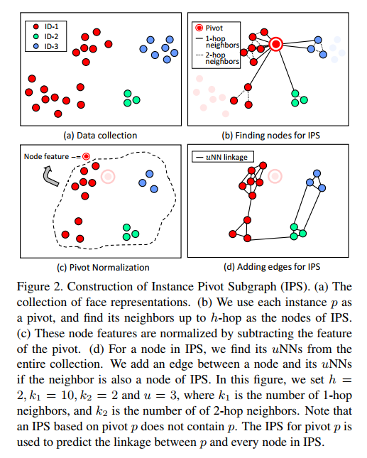

如图，进行到第二步的时候，每个点的状态只有两个，

被 p 连接
成为 2-hop 的 pivot，连接其他点

进行到第三步是标准化，见 3.2.2。 u的解释在最后一步，原文选择了 \(u = 3\)，图中可以发现每个点都连接了 \(\geq 3\) 三次，这是 u 的作用。

在第三步之前，每个点都是被前一层或者 p 点连接的，那么 2-hop 里面的 kNNs 是没有临近点的。因此为了一个闭环的思想，加入了 uNNs，IPS 里面的每个点都可以连接自己的 uNNS。

从实际出发来看，考虑一个 2-hop kNNs 的问题，解决临近点的临近点之间没有连接的问题。这是一个监督学习，y 变量为是否连接，如果出现上述问题，那么模型效果会很差。

3.2.6 Only use 1-hop

The GCN used in this paper is the stack of four graph convolution layers activated by the ReLU function. We then use the cross-entropy loss after the softmax activation as the objective function for optimization.In practice, we only backpropagate the gradient for the nodes of the 1-hop neighbors, because we only consider the linkage between a pivot and its 1-hop neighbors. This strategy not only leads to considerable acceleration compared with the fully super- vised case, but also brings about accuracy gain. The reason is that the high-order neighbors are mostly negative, so the positive and negative samples are more balanced in 1-hop neighbors than in all the neighbors. For testing, we only perform node classification on the 1-hop nodes as well.

因为 high-order-hop kNNs 发现连线过多，样本不平衡了。这里即使是 1-hop 也会做 uNNs 这一步处理。

4 经济学应用

We investigate a disguised form of corruption using a unique and comprehensive sample of credit card data in China. We document that bureaucrats—defined as those working in the government—receive 12% higher credit lines than non-bureaucrats with similar income and demographics.

如果是公务员这个特征，明显给额更高，评级更好，逾期率更低也可以理解。

Despite the higher credit lines, bureaucrats’ credit card accounts experience a higher delinquency rate and a higher likelihood of reinstatement indicating their debt being forgiven by the bank.

但是公务员，给额更高，但是逾期更大，因此这是一种变相腐败。

The effect of greater credit lines and higher delinquency and reinstatement rates associated with bureaucrats is stronger among bureaucrats with a higher hierarchy rank and in more corruptive areas.

并且腐败区域更严重、或者位置更高的公务员群体，逾期和额度关系更紧密(应该说的是相关性更强)。

4.1 Data and Methodology

4.1.1 Data

不可得。

4.1.2 Methodology

\[Y_{i, j, t}=\alpha_{i}+\beta_{i} * \text {Bureaucrat}_{i}+\gamma_{i, j, t} * X_{i, j, t}+\theta_{t}+\delta_{j}+\epsilon_{i, j, t}\]

where \(Y_{i, j, t}\) is the dependent variable denoting the total credit line (or account delinquency indicator, reinstatement indicator, time to reinstatement) granted for individual \(i\) living in city \(j\) at time of credit card origination year \(t .\) Bueaucrats\(_{i}\) is the binary variable equal to one if the applicant works in the government agency. \(X_{i, j, t}\) denotes a vector of demographical controls for the cardholder. \(\theta_{t}\) and \(\delta_{j}\) are time and location fixed effect used to absorb the common variation in time and across locations.

这是一个 longitudinal data。

4.2 Table 1 Summary Statistics

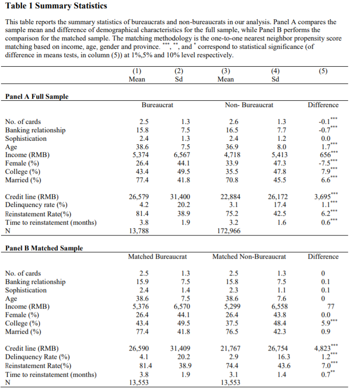
Figure 4.1: panelB 做了一个 PSM 的思想，去查看最相近的样本分是否公务员，查询额度等等的差异。

可以学习 Agarwal et al. (2020) 这里 PSM 的前人综述

4.3 Table 2 The Credit line Premium for Bureaucrats

Sophistication is the total number of banks the individual has established banking relationships through debit card, mortgage loan or credit card account.

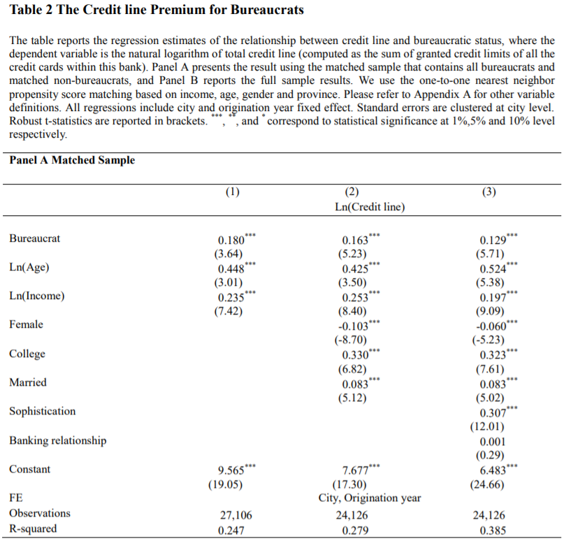
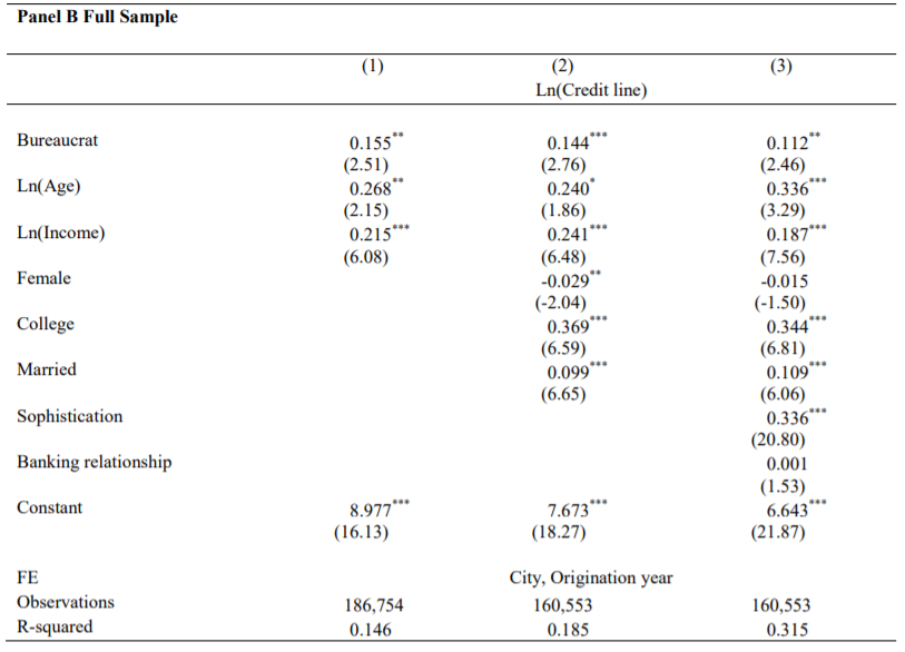
Figure 4.2: 公务员额度更高。‘Sophistication’ 多头反而额度更高。

4.4 Table 3 Cross-sectional Heterogeneity in the Bureaucrat Credit line Premium

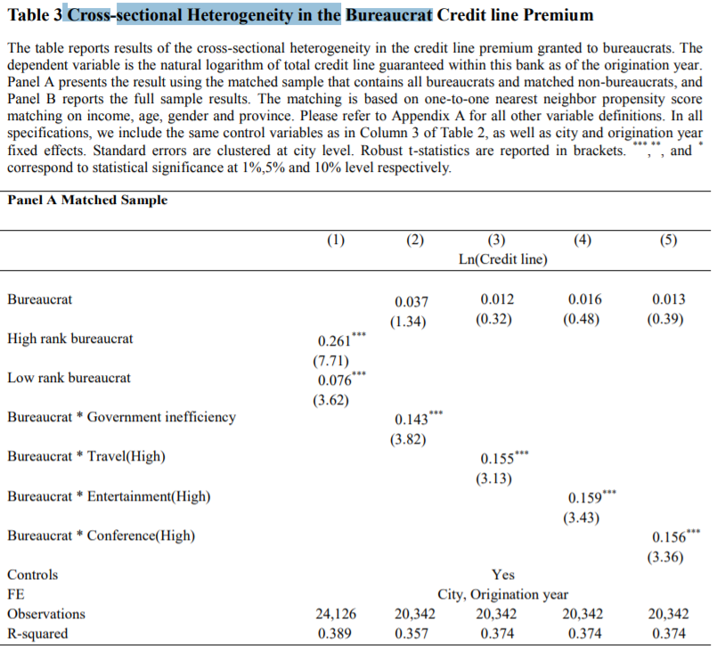
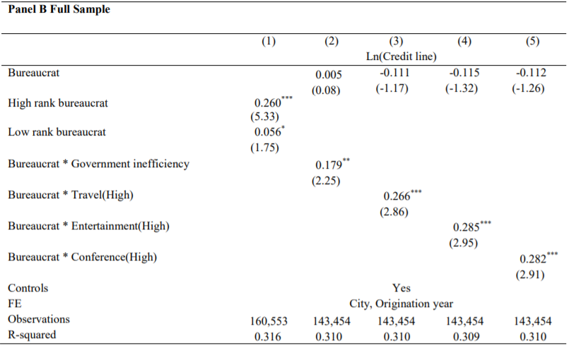
Figure 4.3: ‘Cross-sectional Heterogeneity in the Bureaucrat’ 衡量了公务员之间的差异，’旁骛’更多，额度更高。

Agarwal, Sumit, Wenlan Qian, Amit Seru, and Jian Zhang. 2020. “Disguised Corruption: Evidence from Consumer Credit in China.” Journal of Financial Economics.

Conway, Drew, and John White. 2012. Machine Learning for Hackers Case Studies and Algorithms to Get You Started. O’Reilly Media. http://shop.oreilly.com/product/0636920018483.do.

Hechenbichler, K., and K. Schliep. 2004. “Weighted K-Nearest-Neighbor Techniques and Ordinal Classification.” Sfb386. http://nbn-resolving.de/urn/resolver.pl?urn=nbn:de:bvb:19-epub-1769-9.

Wang, Zhongdao, Liang Zheng, Yali Li, and Shengjin Wang. 2019. “Linkage Based Face Clustering via Graph Convolution Network.”

kNN 学习笔记