空间计量 学习笔记
2020-09-22
- 使用 RMarkdown 的
child参数,进行文档拼接。 - 这样拼接以后的笔记方便复习。
- 相关问题提交到 GitHub
1 检验、模型的流程图
从经典的 OLS 回归开始,我们假设样本之间完全独立。 进而进入面板数据,我们一般拥有 T 和 Id 两个维度,我们创建最近似的OLS回归,叫做 Pooling OLS。 Pooling OLS 回归也是假设样本在 T 和 Id 上都是独立的,历史不影响现在和未来(没有时间相关性),同一时间邻居之间没有影响(没有截面相依性)。 这是一个随机试验的假设,不现实的。
在经济数据集上,数据都是特殊的,比如一个经济时间面板数据,历史影响现在和未来(时间相关性),同一时间邻居之间影响(截面相依性)。 当这个数据是类似于大国数据,那么存在距离的远近,那么影响在距离上存在单调,这就是空间相依性。
但是空间相依性还是比较泛化,不具体,是多个变量之前的相关性。 Moran I 检验更加具体,是单个变量(Y)之间的相关性。
SEM 模型更加具体,只考虑的是 error 项,是 y 在方程中的一部分,所以更加具体。
以上的面板数据都是 T 和 Id,是一种特殊的 longitudinal 数据,更泛化的 longitudinal 数据,可以不用 T。例如 苏丹妮, 盛斌, and 邵朝对 (2019) 采用了地区和行业。
检验的学习是从泛化往具体的,假设更加具体。 数据的收集肯定是特定的,越来越多的收集后,变得泛化。
2 EDA
之前的空间计量部分缺少 EDA 部分,更加直观的理解空间自相关性。 参考 Sparks (2016)
library(spdep)
library(maptools)
library(RColorBrewer)
library(classInt)
dat <-
    readShapePoly(
        "../../data/SA_classdata/SA_classdata.shp",
        proj4string = CRS("+proj=utm +zone=14 +north")
    )

#create a mortality rate, 3 year average
dat$mort3 <-
    apply(dat@data[, c("deaths09", "deaths10", "deaths11")], 1, sum)
dat$mortrate <- 1000 * dat$mort3 / dat$acs_poptot

#get rid of tracts with very low populations
dat <- dat[which(dat$acs_poptot > 100), ]

#Show a basic quantile map of the mortality rate
spplot(
    dat,
    "mortrate",
    main = "Mortality Rate, 3 Year Avg, 2009-2011",
    at = quantile(dat$mortrate),
    col.regions = brewer.pal(n = 5, "Blues")
)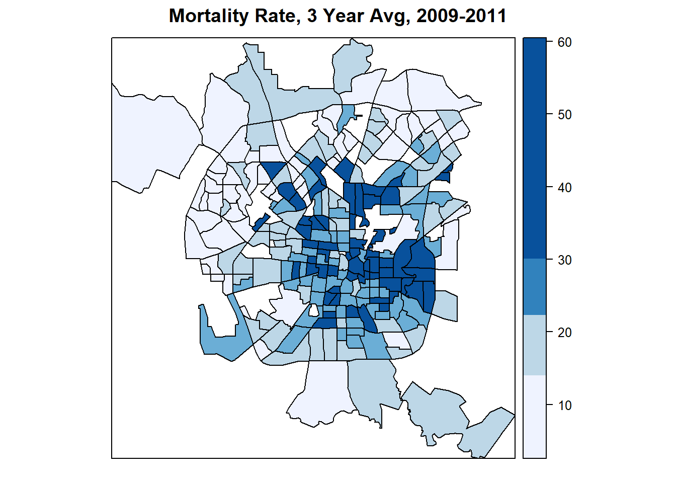
如图展示的是死亡率在地图上的表现,可以发现表现了一定集聚效应(clustering),这是EDA之后要深入的,用统计体现出来。
## Neighbour list object:
## Number of regions: 234
## Number of nonzero links: 1094
## Percentage nonzero weights: 1.997955
## Average number of links: 4.675214
## Link number distribution:
##
## 1 2 3 4 5 6 7 8 9
## 4 11 29 63 68 31 23 3 2
## 4 least connected regions:
## 61 82 147 205 with 1 link
## 2 most connected regions:
## 31 55 with 9 links创建权重矩阵。
salw<-nb2listw(sanb, style="W")
#the style = W row-standardizes the matrix
#make a k-nearest neighbor weight set, with k=3
knn<-knearneigh(x = coordinates(dat), k = 3)
knn3<-knn2nb(knn = knn)这里设置最近的3个地区是相邻,其他为不相邻,这里的k=3可以调节,以深入的理解死亡率的集聚现象。
#generate locally weighted values
wmat<-nb2mat(sanb, style="W")
dat$mort.w<-wmat%*%(dat$mortrate)
#plot the raw mortality rate and the spatiallly averaged rate.
spplot(dat, c("mortrate", "mort.w"),
at=quantile(dat$mortrate),
col.regions=brewer.pal(n=5, "Blues"),
main="Mortality Rate, 3 Year Avg, 2009-2011")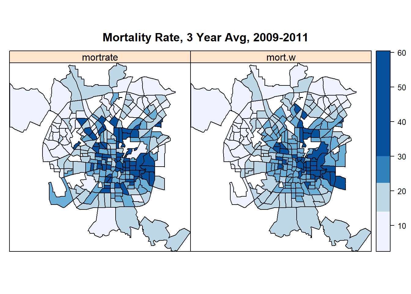
dat$mort.w<-wmat%*%(dat$mortrate)这里是经过空间滞后一期的,更体现了这种集聚现象,可以查看到图片中颜色相似更明显。
以上就是EDA的描述,所以我们需要知道,这两个图的差异大吗?如果差异大,也就是这种空间滞后一期的死亡率差异很大,说明死亡率在该地区空间自相关性很严重,非常受到周边影响。
这需要一个指标来表现,那么就是 Moran I 检验。
##
## Moran I test under randomisation
##
## data: dat$mortrate
## weights: salw
##
## Moran I statistic standard deviate = 10.815, p-value < 2.2e-16
## alternative hypothesis: greater
## sample estimates:
## Moran I statistic Expectation Variance
## 0.472820119 -0.004291845 0.001946053##
## Monte-Carlo simulation of Moran I
##
## data: dat$mortrate
## weights: salw
## number of simulations + 1: 1000
##
## statistic = 0.47282, observed rank = 1000, p-value = 0.001
## alternative hypothesis: greater我查看到是显著的,我们回去参考图,就发现图片的颜色变动还挺大的。 但是我们直观理解下,其实衡量的是死亡率和空间滞后一期的死亡率之间关联度有多大,如果关联度大,Moran I 检验就显著,这其实就是从相关系数中出现的,这里可以画散点图。
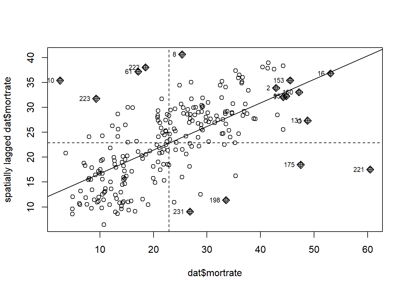
可以看到散点图还是比较能够拟合一条线,这个斜率就是死亡率和空间滞后一期的死亡率之间关联度。 以上就是 Moran I 检验,服务于EDA和描述性统计而已。
What these methods tell you * Moran’s I is a descriptive statistic ONLY, * It simply indicates if there is spatial association/autocorrelation in a variable. (Sparks 2016)
这只是一个描述性统计,因此不需要涉及到模型,只是探查一个变量是否在地理上有空间自相关性。
这是针对于模型的残差而言的,因此属于模型的检验。
这里可以增加一下Moran I 检验在描述性统计中,告诉读者样本中研究变量的空间自相关性,因为是描述性统计所以是不涉及模型的。
简单使用moran.test(var, listw=w)。
不需要使用lm.morantest,这是针对模型、针对残差的。
3 rho 和 weight 的关系
参考 姜磊 (2020, 1:27–31)
\[ Y=\rho C Y+\varepsilon \]
其中 \(CY\) 是自变量,\(\rho\) 是待估计自相关系数,衡量外围地区Y的加权平均之和对中心地区的Y的影响。
\[ \begin{aligned} &C Y=\left(\begin{array}{ccccccccc} \cdots & \cdots & \cdots & \cdots & \cdots & \cdots & \cdots & \cdots & \cdots \\ \vdots & & & & \vdots & & & & \vdots \\ \cdots & \frac{1}{6} & \frac{1}{6} & \frac{1}{6} & 0 & \frac{1}{6} & \frac{1}{6} & \frac{1}{6} & \cdots \\ \vdots & & & & \vdots & & & & \vdots \\ \cdots & \cdots & \cdots & \cdots & \cdots & \cdots & \cdots & \cdots & \cdots \end{array}\right)\left[\begin{array}{c} Y_{i+3}^{*} \\ Y_{i-2} \\ Y_{i-1} \\ Y_{i} \\ Y_{i+1} \\ Y_{i+2} \\ Y_{i+3} \\ \vdots \end{array}\right]\\ &=\left(\frac{1}{6} \times Y_{t-1}+\frac{1}{6} \times Y_{i-2}+\frac{1}{6} \times Y_{i-1}+0+\frac{1}{6} \times Y_{i+1}+\frac{1}{6} \times Y_{i+2}+\frac{1}{6} \times Y_{i+3}\right) \end{aligned} \]
其中\(C\)是\(W\)做了行标准化的,消除某些空间单元影响程度过大。但是只针对于 Rook 临近性决定的,而非空间距离。
\[ L^{s} x_{i}=\sum_{j} w_{i j} x_{j} \]
\[ \boldsymbol{W}=\left(\begin{array}{ccccccccc} \cdots & \cdots & \cdots & \cdots & \cdots & \cdots & \cdots & \cdots & \cdots \\ \vdots & & & & \vdots & & & & \vdots \\ \cdots & 1 & 1 & 1 & 0 & 1 & 1 & 1 & \cdots \\ \vdots & & & & \vdots & & & & \vdots \\ \cdots & \cdots & \cdots & \cdots & \cdots & \cdots & \cdots & \cdots & \cdots \end{array}\right] \]
row index \(i\) 表示中心地区,column index \(j\) 表示外围地区。
但是行标准化并没有具体的数学和统计学理论,并且会增加模型的解释难度。当处理行标准化后,假设有n个相邻,导致权重都变成了1/n。如,河南就有河北、山东、安徽、湖北、陕西和山西决定,但是海南完全被广东决定。
\[ L^{s} x_{i}=\sum_{j} w_{i j} x_{j} \]
并且权重矩阵变成了非对称矩阵。
但是有利于解释实证系数,衡量外围地区Y的加权平均之和对中心地区的Y的影响。
4 空间权重矩阵
4.1 主要分类
0-1(相邻)权重矩阵
0-1(相邻)权重矩阵是根据个体的空间分布来设定权重矩阵的。设定标准为:相邻个体之间取值为 1,不相邻个体为 0
地理距离权重矩阵
基于距离的权重矩阵不仅能衡量相邻个体的相关关系,还能衡量与非相邻个体随距离变化的关系。距离越近,相关程度越高,因此,可以用距离的倒数(\(w_{i j}=\frac{1}{d_{i j}}\))、距离倒数的平方(\(\frac{1}{d_{i}^{2}}\))、或距离N 次方的倒数(\(\frac{1}{d_{i j}^{N}}\))来构造权重矩阵。
参考 王庆喜 (2014, 1:8)
\[W=\left[\begin{array}{cccc} 0 & \frac{1}{\left(d_{1,2}\right)^{2}} & \frac{1}{\left(d_{1,3}\right)^{2}} & \frac{1}{\left(d_{1,4}\right)^{2}} \\ \frac{1}{\left(d_{2,1}\right)^{2}} & 0 & \frac{1}{\left(d_{2,3}\right)^{2}} & \frac{1}{\left(d_{2,4}\right)^{2}} \\ \frac{1}{\left(d_{3,1}\right)^{2}} & \frac{1}{\left(d_{3,2}\right)^{2}} & 0 & \frac{1}{\left(d_{3,4}\right)^{2}} \\ \frac{1}{\left(d_{4,1}\right)^{2}} & \frac{1}{\left(d_{4,2}\right)^{2}} & \frac{1}{\left(d_{4,3}\right)^{2}} & 0 \end{array}\right]\]
经济距离权重矩阵
经济距离权重矩阵可以用两个地区人均GDP之差绝对值的倒数来衡量。两个地区经济发展水平相似,权重就较大;如果两个地区发展水平差距大,其权重就较小 当\(i \neq j\)时,\(w_{i j}=\frac{1}{\left|\bar{Y}_{i}-\bar{Y}_{j}\right|}\) 此权重矩阵的缺陷为\(W_{i j}=W_{j i}\),经济发展较好的区域对较差区域的影响,一般会大于经济较差地区对经济较好地区的影响,但是这种差异并没有反应出来。
基于贸易的权重矩阵
基于贸易的权重矩阵,能够衡量各国间经济联系情况,体现了国际外溢性,它可以用两个国家或地区间的贸易额来衡量。两个国家间的贸易越频繁,权重就越大; 当\(i \neq j\)时,\(w_{i j}=\text {trade}_{i j}\)
基于投入产出表的权重矩阵(借鉴意义小)
基于投入产出表的权重矩阵可以用来表示产业间的相互联系,对一个产业的冲击会通过各产业间的投入产出关系对其他产业产生影响,这也是产业的外溢性。 与其他权重矩阵不同的是,没有经过行标准化的投入产出权重矩阵不再是对称矩阵,其主对角线上的元素也不再为0。 主要是对产业的冲击,因此我们不太能用到这个。
社会经济结构的空间权重矩阵
姜磊 (2020) 的文章定义了社会经济结构的空间权重矩阵,其基本形式如下: \[w_{i j}=\left\{\begin{array}{l} \frac{1}{\left|\bar{Y}_{i}-\bar{Y}_{j}\right|} \\ 0 \end{array}\right.\]
\[\overline{Y_{i}}=\frac{1}{t_{1}-t_{0}+1} \sum_{t=t_{0}}^{t_{1}} Y_{i t}\]
需要注意的是,这里的空间权重矩阵是内生的。
时变空间权重矩阵
姜磊 (2020) 认为地理是不随时间变化而变化的。但如果考察对象是社会经济情况或人口地理的分布特征,这种空间效应如\(W_{i t}\) 或者 \(\rho\) 是会随时间变化的。 姜磊 (2020) 列举了GDP构造差异、人口的死亡、出生或迁移行为的例子,其基本形式如下: \[y=\rho W_{i t}+\tau y_{i-1}+\delta W_{i} y_{\mu-1}+X \beta+\mu_{i}+\gamma_{i}+\varepsilon_{i}\] 其中,\(W_{i t}\) 表示随时间变化的空间权重矩阵。
权重矩阵的混合使用(借鉴意义小)
以上权重矩阵可以根据研究需要混合使用,也可以稍加变形满足研究需要。以下以地理经济距离权重矩阵为例。 \[W=W_{d} \cdot\left(\begin{array}{c} \bar{Y}_{1} \\ \bar{Y} \\ \bar{Y}_{2} \\ \bar{Y} \\ \cdots \\ \bar{Y}_{n} \\ \bar{Y} \end{array}\right)\] Wd是地理距离矩阵,\(\bar{Y}_{i}=\frac{1}{t_{1}-t_{0}+1} \sum_{i_{0}}^{i} Y_{i j}\)为各省人均GDP均值,\(\bar{Y}_{i}=\frac{1}{n\left(t_{1}-t_{0}+1\right)} \sum_{i=1}^{n} \sum_{t_{0}}^{t_{1}} Y_{i t}\)为全国人均GDP均值。此权重矩阵为非对称矩阵,它克服了上述一般经济距离权重矩阵的缺陷,使经济发达地区对经济不发达地区的影响,大于经济不发达对经济发达地区的影响。
为了对理论分析部分提出的两个假设进行检验,本文在借鉴 LeSage and Pace(2009) 提出的空间杜宾模型基础上,构建如下两个模型进行实证分析:
\[\begin{array}{r} B g_{i t}=\alpha+\rho_{1} d W B g_{i t}+\rho_{2}(1-d) W B g_{i t}+\beta T c_{i t}+\gamma W T c_{i t}+\theta \ln I c_{i t}+\delta W I c_{i t} \\ +\sum_{n=1}^{N} \lambda_{n} X_{n i t}+\mu_{i}+v_{t}+\varepsilon_{i t} \\ B e_{i t}=\alpha+\rho W B e_{i t}+\beta\left(T c_{i t} \times B d_{i t}\right)+\gamma W\left(T c_{i t} \times B d_{i t}\right)+\theta\left(I c_{i t} \times B d_{i t}\right)+\delta W\left(I c_{i t} \times B d_{i t}\right) \\ +\sum_{n=1}^{N} \lambda_{n} Y_{n i t}+\mu_{i}+v_{t}+\varepsilon_{i t} \end{array}\]
其中\(d\)和\(1-d\)不对称,更加具备经济解释。
其中,式( 12)用于对假设 1, 即地方竞争对地方政府举债行为策略的影响进行识别和 实证检验。在式( 12 ) 中被解释变量 \(Bg_{it}\) 是地区 \(i\) 在 \(t\) 年的地方政府债务规模增速,解释变量 \(T c_{i}\) 和 \(I c_{i}\) 分别是地区 \(i\) 在 \(t\) 年的税收竞争和公共投资竞争,\(W\) 代表空间权重矩阵, \(X_{n i t}\) 代表控制变量。此外, \(d\) 代表虚拟变量,当与相邻地区相比,本地区 GDP 增速相对较低时,取值为 1,反之,当本地区 GDP 增速相对较高时,取值为 0。之所以采取虚拟变量, 主要是本地区地方效用函数在很大程度上会受相邻地区 GDP 的影响。与此同时,对于模 型变量的估计系数来说, \(\rho_{1}、\rho_{2}\) 代表被解释变量的空间滞后项系数,其中, \(\rho_{1}\) 代表本地区 GDP 增速落后时,相邻地区地方政府举债行为策略对于本地区的影响, 而 \(\rho_{2}\) 代表本地区 GDP 增速领先时的相应影响。\(\gamma\) 和 \(\delta\) 代表两个解释变量的空间滞后项系数。
可以学习\(\rho_{1}、\rho_{2}\) 代表被解释变量的空间滞后项系数的处理,这样的话,我们可以把 GDP 和 地理权重矩阵进行乘积,按照 洪源, 陈丽, and 曹越 (2020) 的处理,更有经济解释。
(13)用于对假设 2,即地方竞争对于地方政府债务绩效的影响进行识别与实证检验。在式(13)中被解释变量 \(Be_{it}\) 是地区 \(i\) 在 \(t\) 年的地方政府债务绩效,解释变量 \(T c_{i t} \times\) \(B d_{i t}\) 和 \(I c_{i t} \times B d_{i t}\) 分别是地区 \(i\) 在 \(t\) 年的税收竞争与地方政府负债率的交互项和公共投资 竞争与地方政府负债率的交互项。之所以采取交互项变量,主要因为地方竞争影响债务 绩效的方向和程度与地方政府债务既定存量规模水平有密切关联,因而希望通过交互项 设置,反映出在地方政府采取举债策略形成相应债务存量水平的情况下,地方竞争对于债 务绩效的具体影响。\(Y_{nit}s\) 代表控制变量。
理解交互项的经济解释。
4.2 社会经济结构的空间权重矩阵
参考 姜磊 (2020)
\[ w_{i j}=\left\{\begin{array}{l} \frac{1}{\left|\bar{Y}_{i}-\bar{Y}_{j}\right|} \\ 0 \end{array}\right. \]
\[ \overline{Y_{i}}=\frac{1}{t_{1}-t_{0}+1} \sum_{t=t_{0}}^{t_{1}} Y_{i t} \]
这里要注意,这里的空间权重矩阵是内生的。
5 Spatial Correlation
5.1 Testing for Spatial Dependence
5.1.1 CD p Tests for Local Cross-sectional Dependence
参考 Pesaran (2004) 对 \(\rho\) 的汇总处理。
\[\mathbf{C D}=\sqrt{\frac{1}{\sum_{n=1}^{N-1} \sum_{m=n+1}^{N} w(p)_{n m}}}\left(\sum_{n=1}^{N-1} \sum_{m=n+1}^{N}[w(p)]_{n m} \sqrt{T_{n m} \hat{\rho}_{n m}}\right)\]
CD test 我们在之前的截面相依性接触过。这里是一个改进版本。注意 \([w(p)]_{n m}\),当两个个体不是相邻时,两者之间的相关性就不会被计入,因此这个调整过的 CD(p) test 引入邻近矩阵后,具备了空间相关性的度量。
## ALABAMA ARIZONA ARKANSAS CALIFORNIA COLORADO CONNECTICUT
## ALABAMA 0 0.0000000 0 0.0 0.0 0
## ARIZONA 0 0.0000000 0 0.2 0.2 0
## ARKANSAS 0 0.0000000 0 0.0 0.0 0
## CALIFORNIA 0 0.3333333 0 0.0 0.0 0
## COLORADO 0 0.1428571 0 0.0 0.0 0
## CONNECTICUT 0 0.0000000 0 0.0 0.0 0##
## Pesaran CD test for local cross-sectional dependence in panels
##
## data: php$price
## z = 37.288, p-value < 2.2e-16
## alternative hypothesis: cross-sectional dependence5.1.2 The Randomized W Test
The rw test of Millo (2017) employs a permutation procedure to produce a large number of randomized neighborhood matrices and then compares the cd(p) statistic under the true spatial ordering with the population of those under the randomized ones.
思路上,RW Test 其实是对 CD(p) test 进行模拟仿真,查看是否满足普遍情况。
The idea underlying the cd(p) test, that not all pairs of neighbors are correlated but only those in a specific spatial relationship are and that the latter are identified through the W matrix, gives rise to another testing procedure that is remarkably robust to all the above confounding features.
CD(p) Test 其实检验的是局部个体间的空间相依性,因为只有\([w(p)]_{n m}=1\)的个体之间才考虑空间相依性,因此空间相依性不是一个全局的考虑,并且度量非常受制于邻近矩阵的设定。 Millo (2017) 的操作方式是将 \([w(p)]_{n m}=1\) 随机打乱,制造若干个随机后的邻近矩阵,理论上如果是随机的,那么随机出来的邻近矩阵也还是能够计算出空间相依性,那么就说明原先靠局部个体计算的空间相依性是不显著的,不能代表整体,并且轻易的被随机出来的邻近矩阵体现出来。
An rw test will determine whether there is any spatial correlation proper left after controlling for cross-sectional correlation.
并且这种随机性,得到的空间相依性是条件的,去除了截面相依性。
\[\mathrm{p} \text { -value }^{*}\left(\mathbf{R} \mathbf{w}_{p}^{+}\right)=\frac{\sum_{h=1}^{B} 1\left[\tau_{h}^{*} \geq \hat{\tau}\right]}{B+1}\]
- \(\hat{\tau}=\mathbf{c} \mathbf{D}_{p}(W | x)\) 是靠真实的邻近矩阵计算的CD统计值
- \(\tau_{h}^{*}=\mathbf{C D}_{p}\left(W_{h}^{*} | x\right)\) 是靠随机的邻近矩阵计算的CD统计值,\(B\)是迭代次数
以上情况没有考虑空间相依性是负的情况,因此产生
\[\mathrm{p} \text { -value }^{*}\left(\mathbf{R} \mathbf{w}_{p}^{s y m m}\right)=\frac{\sum_{h=1}^{B} 1\left[\left|\tau_{h}^{*}\right| \geq|\hat{\tau}|\right]}{B+1}\]
考虑到统计值分布是不对称的情况,因此产生
\[\mathrm{p} \text { -value }^{*}\left(\mathbf{R} \mathbf{w}_{p}\right)=2 \times \min \left(\frac{\sum_{h=1}^{B} 1\left[\tau_{h}^{*} \leq \hat{\tau}\right]}{B+1}, \frac{\sum_{h=1}^{B} 1\left[\tau_{h}^{*}>\hat{\tau}\right]}{B+1}\right)\]
##
## Randomized W test for spatial correlation of order 1
##
## data: formula
## p-value = 0.002
## alternative hypothesis: twosidedreplications 代表了 B,也就是迭代过程。
5.2 残差情况
以上考虑的是变量,同时可以考虑对模型的残差进行检验。
mgmod <- pmg(log(price) ~ log(income), data = HousePricesUS)
ccemgmod <- pmg(log(price) ~ log(income), data = HousePricesUS, model = "cmg")
pcdtest(resid(ccemgmod), w = usaw49)##
## Pesaran CD test for local cross-sectional dependence in panels
##
## data: resid(ccemgmod)
## z = 28.217, p-value < 2.2e-16
## alternative hypothesis: cross-sectional dependence##
## Randomized W test for spatial correlation of order 1
##
## data: formula
## p-value = 0.002
## alternative hypothesis: twosided6 三种空间交互效应以及引申的八种模型
参考 姜磊 (2020, 1:章节5.1.3)
- endogenous interaction effects \(y_i \to y_j\) SLM 空间滞后模型
- exogenous interaction effects \(x_i \to y_i\) SLX 空间自变量滞后模型
- interaction effects in the residuals \(\varepsilon_i \to \varepsilon_j\) SEM 空间误差模型
- SDM = SLM + SLX 杜宾模型
- SDEM = SEM + SLX 杜宾误差模型
- SAC = SLM + SEM KPM Kelejian-Prucha 模型
- GNSM = SLM + SLX + SEM general nesting spatial model 一般嵌套空间模型
因此会引申出以上八个模型(加上 OLS),这会在我们的实证中都包含,进而进行交叉比较。
7 Spatial Lags
The basic tool of spatial econometrics is the definition of a spatial lag.
spatial lag 是关键词,类似于 time series 中的 time lag,这是空间计量的核心。
\[y=\lambda\left(\mathrm{I}_{T} \otimes W_{N}\right) y+Z \gamma+\epsilon\]
7.1 SLM
参考 姜磊 (2020, 1:章节5.3.1)
\[ y=\rho W y+X \beta+\varepsilon \]
\(\rho\)和\(\beta\)才是待估计的。
This is called the spatial lag model proper. From a theoretical viewpoint, it is appropriate whenever one expects the outcome of one observation to influence the outcomes of neighboring ones, such as, e.g., for the spreading of a disease, where one unit being positive has a direct effect on the likelihood of neighboring units to be so too.
在空间上,一个邻居对另外一个邻居的影响,是 xxx unit 的。 类似于时间序列模型中,滞后一期对因变量的影响的解读。
In a microeconomic setting, the effect of a spatial lag term could be expected to turn out positive is in copycatting behavior, when e.g., buying a product sparks imitation hereby raising the propensity of neighbors to follow suit. A negative spatial lag can instead be consistent with the idea of free riding: if one can reap advantage from the actions of neighbors through some kind of externality, then this will lower his or her own effort
- 这可以体现出从众效应,当一个企业购买了一个2B的产品,其他同行业的企业也会跟从。
- 这可以体现搭便车效应,当一个人提供了服务,其他将不这样做,节省力气。
library(plm)
library(splm)
library(lmtest)
data("Cigar", package = "plm")
fm <- log(sales) ~ log(price) + log(pimin) + log(ndi / cpi)
femod <- plm(fm, Cigar)
coeftest(femod)##
## t test of coefficients:
##
## Estimate Std. Error t value Pr(>|t|)
## log(price) -0.751306 0.046169 -16.273 < 2.2e-16 ***
## log(pimin) 0.494602 0.045617 10.843 < 2.2e-16 ***
## log(ndi/cpi) 0.680070 0.036753 18.504 < 2.2e-16 ***
## ---
## Signif. codes: 0 '***' 0.001 '**' 0.01 '*' 0.05 '.' 0.1 ' ' 1这里没有控制空间 lags。
cig <-
Cigar %>%
arrange(year, state)
wp <-
kronecker(diag(1, 30), wcig) %*% cig$price # price spatial lags
cig <-
cig %>%
mutate(wp = wp[order(cig$state, cig$year)])##
## t test of coefficients:
##
## Estimate Std. Error t value Pr(>|t|)
## log(price) -0.263039 0.010130 -25.9656 < 2e-16 ***
## log(ndi/cpi) 0.683275 0.038309 17.8358 < 2e-16 ***
## log(wp) 0.098898 0.048577 2.0359 0.04196 *
## ---
## Signif. codes: 0 '***' 0.001 '**' 0.01 '*' 0.05 '.' 0.1 ' ' 1可以发现 spatial lag 是显著的。
毕竟 spatial lag 是 WX 矩阵相乘即可,因此有更方便的输入方式。
lwcig <- mat2listw(wcig)
fm3 <- update(fm, . ~ . - log(pimin) +
log(slag(price, listw = lwcig)))
femod3 <- plm(fm3, Cigar)
coeftest(femod3)##
## t test of coefficients:
##
## Estimate Std. Error t value Pr(>|t|)
## log(price) -0.829249 0.052807 -15.703 < 2.2e-16 ***
## log(ndi/cpi) 0.629425 0.037093 16.969 < 2.2e-16 ***
## log(slag(price, listw = lwcig)) 0.587352 0.053739 10.930 < 2.2e-16 ***
## ---
## Signif. codes: 0 '***' 0.001 '**' 0.01 '*' 0.05 '.' 0.1 ' ' 1Wy is endogenous by construction, and therefore the estimator is hopelessly biased;
这里需要注意的是,\(Wy\) 是内生的,因此直接用 OLS 回归,得到的结果是 biased。
7.2 Spatial OLS
SAR (spatially autoregressive) (Franzese and Hays 2007) 是空间计量最基础的模型,因此和 OLS 看起来很类似,但是因为加入的是内生性交互效应
\[ y=(\boldsymbol{I}-\rho \boldsymbol{W})^{-1} \boldsymbol{X} \boldsymbol{\beta}+(\boldsymbol{I}-\rho \boldsymbol{W})^{-1} \boldsymbol{\varepsilon} \]
所以\(Wy\)和\(\boldsymbol{\varepsilon}\)是不独立的(姜磊 2020, 1:章节5.3.3),因此不可以直接把 \(Wy\)作为回归因子做OLS回归,因此 OLS 估计有偏且不一致,换成
- ML 极大似然估计,QML 伪极大似然估计
- IV,GMM
- BMC-MC
7.3 Moran I 和 SAR 的关系
Since spatial data often display correlations amongst closely located observations (autocorrelation), we should probably test for autocorrelation in the model residuals, as that would violate the assumptions of the OLS model. One method for doing this is to calculate the value of Moran’s I for the OLS residuals. (Sparks 2016)
空间自相关性的检验一种是从 Moran I 检验查看,一种是直接跑空间计量模型查看对应指标的显著性。
This autoregression introduces dependence into the data. Instead of specifying the autoregression structure directly, we introduce spatial autocorrelation through a global autocorrelation coefficient and a spatial proximity measure. (Sparks 2016) To account for the expected spatial association in the data, we would like a model that accounts for the spatial structure of the data. One such way of doing this is by allowing there to be correlation between residuals in our model, or to be correlation in the dependent variable. (Sparks 2016)
两者的思路差异为
Theorem 7.1 空间自相关模型是假设模型残差不是独立同分布假设,而是空间自相关性,然后建模后看是否显著
One such way of doing this is by allowing there to be correlation between residuals in our model, or to be correlation in the dependent variable. (Sparks 2016)
Theorem 7.2 Moran I 检验是假设残差是独立同分布假设,然后建模后对 \(\mu\) 进行检查是否有空间自相关性
We saw in the normal OLS model that some of the basic assumptions of the model are that the: 1) model residuals are distributed as iid standard normal random variates 2) and that they have common (and constant, meaning homoskedastic) unit variance. (Sparks 2016)
因此 结论 7.2 和 结论 7.1 两者的目的相同,但是结论不是互相支持的。 满足结论 7.2并不一定满足结论7.1。因此这是两个殊途同归的方法,存在互补性不是替代性。
检验 OLS 残差是否有空间相依性,所以一开始要先估计 OLS,是空间计量的开始(姜磊 2020, 1:章节5.4.1),关于 OLS 和空间计量的关系参考章节 6。
7.4 Moran I 检验在 residual 的效果
参考章节 2,我们对死亡率一个变量进行了 Moran I 检验和实际地图的探索,这是一种很好的方式,可以理解 Moran I 检验的显著性和最后图像的改变的差异。
参考 Sparks (2016)
library(spdep)
library(maptools)
library(RColorBrewer)
dat<-readShapePoly("../../data/SA_classdata/SA_classdata.shp", proj4string=CRS("+proj=utm +zone=14 +north"))
#Make a rook style weight matrix
sanb<-poly2nb(dat, queen=F)
summary(sanb)
## Neighbour list object:
## Number of regions: 235
## Number of nonzero links: 1106
## Percentage nonzero weights: 2.002716
## Average number of links: 4.706383
## Link number distribution:
##
## 1 2 3 4 5 6 7 8 9
## 4 10 30 62 66 34 24 3 2
## 4 least connected regions:
## 61 82 147 205 with 1 link
## 2 most connected regions:
## 31 55 with 9 linkssalw<-nb2listw(sanb, style="W")
wmat<-nb2mat(sanb, style="W")
fit2<-lm(I(viol3yr/acs_poptot) ~ pfemhh + hwy + p5yrinmig + log(MEDHHINC), data=dat )
dat$resid<-rstudent(fit2)
dat$resid.w<-wmat%*%(dat$resid)
spplot(dat, c("resid", "resid.w"),
at=quantile(dat$resid),
col.regions=brewer.pal(n=5, "RdBu"),
main="Residuals from OLS Fit of Crime Rate")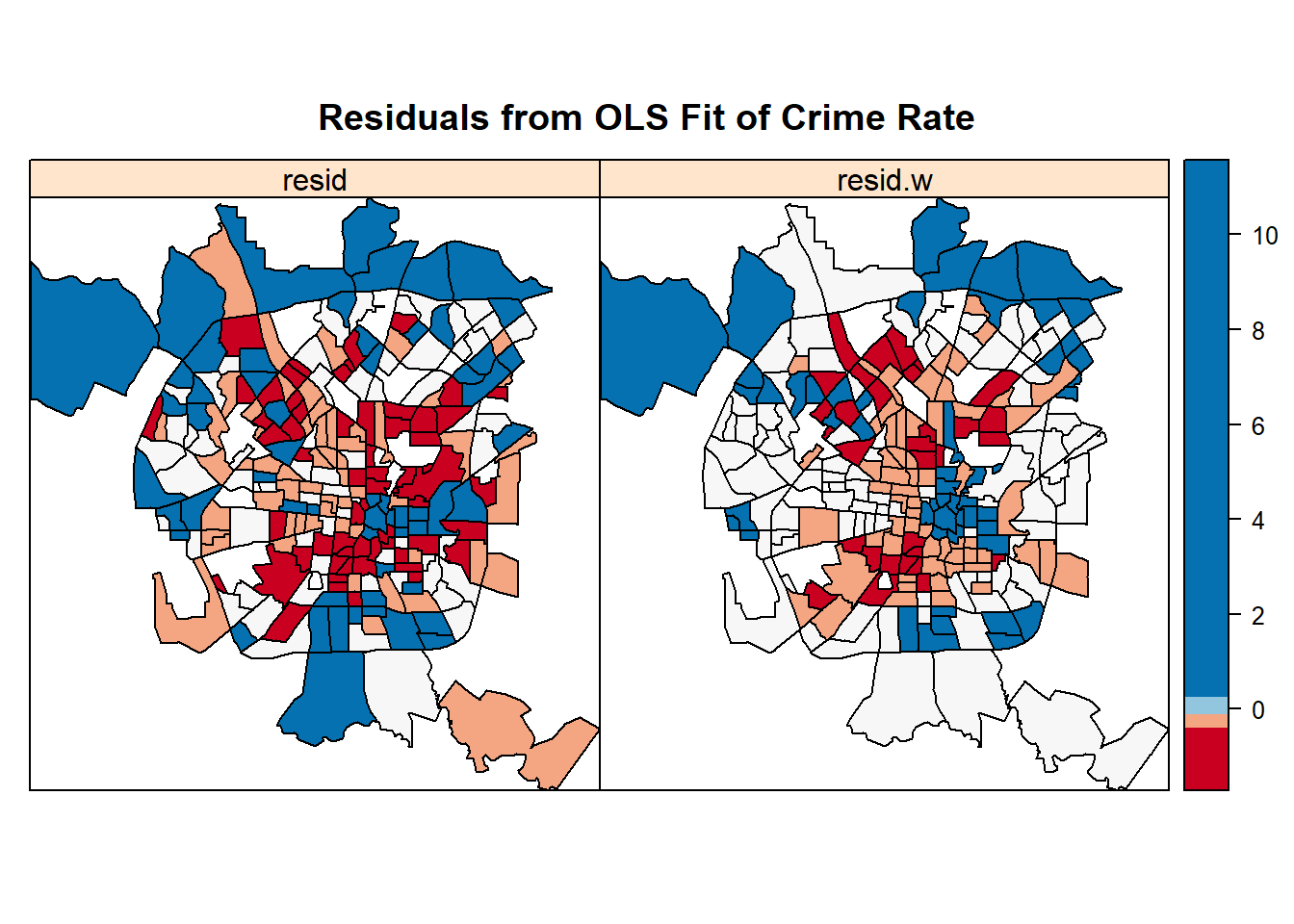
我们可以查询到图像中间区域的颜色变动差异不大。
##
##  Global Moran I for regression residuals
##
## data:
## model: lm(formula = I(viol3yr/acs_poptot) ~ pfemhh + hwy + p5yrinmig + log(MEDHHINC), data = dat)
## weights: salw
##
## Moran I statistic standard deviate = 0.75475, p-value = 0.2252
## alternative hypothesis: greater
## sample estimates:
## Observed Moran I      Expectation         Variance
##      0.021326432     -0.011406176      0.001880845
因此我们可以看到Moran I检验差异不大。
residuals lm.morantest检测结果并不显著,是比较常见的。
7.5 SEM
Te other main specification in the literature, the spatial error, is instead appropriate when one expects the innovation relative to one observation to influence the outcomes of neighboring ones. (Sparks 2016)
SEM 是针对 error 进行研究的,在计量中,因为 error 是不受到自变量约束的,因此常作为 y 变量的 innovation,也就是创新项目,基本假设是,创新不受到目前可控的 x 影响。
Millo (2014) 给定定义
\[y=Z \gamma+\epsilon\] \[\epsilon=\rho W \epsilon+v\]
data("RiceFarms", package = "splm")
data("riceww", package = "splm")
library(spdep)
library(plm)
library(splm)
ricelw <- mat2listw(riceww)
Rice <- pdata.frame(RiceFarms, index = "id")
riceprod <-
log(goutput) ~ log(seed) + log(totlabor) + log(size) + region + time
rice.sem <- spreml(
riceprod,
data = Rice,
w = riceww,
lag = FALSE,
errors = "sem"
)
summary(rice.sem)## ML panel with , spatial error correlation
##
## Call:
## spreml(formula = riceprod, data = Rice, w = riceww, lag = FALSE,
## errors = "sem")
##
## Residuals:
## Min. 1st Qu. Median 3rd Qu. Max.
## -1.0685835 -0.2329965 0.0058127 0.2348086 1.4896241
##
## Error variance parameters:
## Estimate Std. Error t-value Pr(>|t|)
## rho 0.562689 0.051773 10.868 < 2.2e-16 ***
##
## Coefficients:
## Estimate Std. Error t-value Pr(>|t|)
## (Intercept) 5.8541287 0.1946926 30.0686 < 2.2e-16 ***
## log(seed) 0.1662622 0.0247465 6.7186 1.835e-11 ***
## log(totlabor) 0.2482188 0.0275843 8.9985 < 2.2e-16 ***
## log(size) 0.5977627 0.0279975 21.3505 < 2.2e-16 ***
## regionlangan -0.0977908 0.0913709 -1.0703 0.28450
## regiongunungwangi -0.1404809 0.0842233 -1.6680 0.09532 .
## regionmalausma -0.1186456 0.0865045 -1.3716 0.17020
## regionsukaambit 0.0072316 0.0937222 0.0772 0.93850
## regionciwangi -0.0138065 0.0846467 -0.1631 0.87043
## time2 -0.0474541 0.0788454 -0.6019 0.54727
## time3 -0.1855069 0.0788642 -2.3522 0.01866 *
## time4 -0.3472240 0.0788324 -4.4046 1.060e-05 ***
## time5 0.1581838 0.0788594 2.0059 0.04487 *
## time6 0.1380488 0.0788065 1.7517 0.07982 .
## ---
## Signif. codes: 0 '***' 0.001 '**' 0.01 '*' 0.05 '.' 0.1 ' ' 1rho 很显著,说明地区之间的 error 非常空间相依。
8 Individual Heterogeneity
To solve the problem, Lee and Yu (2010 Chapter 3.2) suggest either a different orthonormal transformation of the data or an ex-post correction of the estimated variance (Lee and Yu 2012).
类似于我们考虑 pooling OLS 和 FE 等的区别,就是去度量个体效应,这一块就是讨论这部分模型。
8.1 Spatial Panel Models with Error Components
\[y=\lambda\left(\mathrm{I}_{T} \otimes W_{N}\right) y+Z \gamma+\epsilon\] \[\epsilon=\left(j_{T} \otimes I_{N}\right) \eta+v\] \[v=\rho\left(\mathrm{I}_{T} \otimes W_{N}\right) v+\zeta\]
Following the treatment in Millo (2014), on which this part of the chapter is based, we label the combined model containing both a spatial lag and a spatial error process SAREM. (This is also often called SARAR, because of the two spatial autoregressive processes, one in the response and one in the errors.
Lee and Yu (2012 Chapter 2.4) illustrate the difference between this latter specification and semre through the likelihood of the between model. We label this latter alternative specification SEM2RE, and its extension to including a spatial lag (Mutl and Pfaffermayr 2011) SAREM2RE.
基于 Spatial OLS,后面衍生了模型,
- SAREM (SARAR)
- SEM2RE
- SAREM2RE
8.2 Locally Robust Spatial LM Tests
参考 姜磊 (2020, 1:章节5.5.1) 判断用 SLM 还是 SEM,满足
\[\text{LM-lag} + \text{robust LM-error} = \text{LM-error} + \text{robust LM-lag}\]
- Robust LM-error 高,选择 SEM
- Robust LM-lag 高,选择 SLM
\[ \mathrm{LM}-\operatorname{lag}=\frac{\left[e^{\mathrm{T}} W y / \sigma^{2}\right]^{2}}{J} \]
\[ J=\frac{1}{\sigma^{2}}(W X \beta)^{\mathrm{T}}\left[I-X\left(X^{\mathrm{T}} X\right)^{-1} X^{\mathrm{T}}\right](W X \beta)+T_{\mathrm{w} \sigma^{2}} \]
\(e\) 是 OLS 回归的残差项。
\[ T_{W}=\operatorname{tr}\left[\boldsymbol{W} \boldsymbol{W}+\boldsymbol{W}^{\mathrm{T}} \boldsymbol{W}\right] \]
\[ \begin{aligned} &\text { robust LM-lag }=\frac{\left[e^{T} W y / \sigma^{2}-e^{T} W e / d^{2}\right]^{2}}{J-T_{W}}\\ &\text { robust LM-error }=\frac{\left[e^{T} W e / \sigma^{2}-T_{w} e^{T} W y / \sigma^{2}\right]^{2}}{T_{w}\left[1-T_{w} / J\right]} \end{aligned} \]
The robust LM tests of Anselin et al. (1993) can, in turn, be straightforwardly adapted to the (pooled) panel case.
\[\begin{array}{l}{R \mathrm{LM}_{\rho | \lambda}=\frac{\left.\left(\hat{\epsilon}^{\top}\left(\mathrm{I}_{T} \otimes W\right) y / \hat{\sigma}_{\epsilon}^{2}\right)^{2}-\hat{\epsilon}^{\top}\left(\mathrm{I}_{T} \otimes W\right) \hat{\epsilon} / \hat{\sigma}_{\epsilon}^{2}\right)^{2}}{J-T T_{W}}} \\ {R \mathrm{LM}_{\lambda | \rho}=\frac{\left.\left(\hat{\epsilon}^{\top}\left(\mathrm{I}_{T} \otimes W\right) \hat{\epsilon} / \hat{\sigma}_{\epsilon}^{2}\right)^{2}-T T_{W} / J \hat{\epsilon}^{\top}\left(\mathrm{I}_{T} \otimes W\right) y / \hat{\sigma}_{\epsilon}^{2}\right)^{2}}{T T_{W}\left(1-T T_{W} / J\right)}}\end{array}\]
8.3 Wald Tests
怀特检验,比较简单。
\[\text { Wald }_{\rho | \lambda}=\frac{\hat{\rho}}{\sqrt{\hat{V}(\hat{\rho})}} \sim N(0,1)\]
9 Serial and spatial Correlation
类似于之前查看截面相依性和自相关性时一样,两种相关性会互相影响,不独立,因此查看共同的检验是有必要的。
As an alternative to the saremsrre specification, Millo (2014) presents an extension of the SEM2RE errors a Kapoor, Kelejian, and Prucha (2007) to serial correlation in the remainder errors. As in the SEM2RE case, the random effects are spatially lagged together with the idiosyncratic ones, while the remaining errors \(\epsilon\), in turn, are serially correlated:
\[\begin{aligned} y &=\lambda\left(\mathrm{I}_{T} \otimes W\right) y+Z \gamma+\epsilon \\ \epsilon &=\left(j_{T} \otimes \eta\right)+v \\ \epsilon &=\rho\left(\mathrm{I}_{T} \otimes W\right) \epsilon+\zeta \\ \zeta_{t} &=\psi \zeta_{t-1}+\xi_{t} \end{aligned}\]
SEM2RE 可以了解下。
9.1 Tests for Random Effects, Spatial, and Serial Error Correlation
Baltagi et al. (2007) derive the joint, marginal, and conditional lm tests for the model with serial correlation.
关注下 Baltagi et al. (2007) 这篇文献。
10 SLX 和外部性
WX 就是外部性,所以 SLX 就是专门度量外部性的。 同理,就是在OLS 回归中加入这个外生变量(姜磊 2020, 1:章节5.8.1)。
如房价受到很房龄、质量、面积等,还受到周围垃圾处理厂、学校、医院影响,这些就是外部性。
\[ y=X \beta+W X \theta+\varepsilon \]
11 Kelejian-Prucha 模型
也叫作 KPM,等于 SLM 和 SEM 的合成。(姜磊 2020, 1:章节5.9)
\[ \left\{\begin{array}{l} y=\rho W y+X \beta+\varepsilon \\ \varepsilon=\lambda W \varepsilon+v \end{array}\right. \]
\(W\) 也可以不同,于是
\[ \left\{\begin{array}{l} y=\rho W_{1} y+X \beta+\varepsilon \\ \varepsilon=\lambda W_{2} \varepsilon+v \end{array}\right. \]
也叫作SARMA(1,1)=KPM
\[ \left\{\begin{array}{l} y=\rho_{1} W_{1} y+\rho_{2} W_{2} y+\rho_{3} W_{3} y+\cdots+\rho_{\rho} W_{\rho} y+X \beta+\varepsilon \\ \varepsilon=\varphi_{1} W_{1} \varepsilon+\varphi_{2} W_{2} \varepsilon+\varphi_{3} W_{3} \varepsilon+\cdots+\varphi_{q} W_{q} \varepsilon+v \end{array}\right. \]
\[ \begin{array}{c} A Y=\alpha+B \varepsilon \\ A=I-\sum_{j=1}^{p} \rho W^{j} ; B=I+\sum_{j=1}^{q} \varphi W^{j} \end{array} \]
12 SDM
- 模型的优势在于即使数据生成是 SLM 或者 SEM,SDM 估计也是无偏的
- 因此对于 x 的交互效应并未强加先验的约束条件,因此统计不显著,可以再提出,这样也不存在变量遗漏问题(姜磊 2020, 1:章节5.6)
\[ y=\rho W y+X \beta+W X \theta+\varepsilon \]
\(\theta\) 是待估计的。比如研究经济增长的模型考虑人力资本,考虑北京的经济增长时,既要考虑北京毕业生留在北京的,河北的也会,因此需要把河北控制住,否则遗漏变量了。
If you remember, one issue that commonly occures with the lag model, is that we often have residual autocorrelation in the model. This autocorrelation could be attributable to a missing spatial covariate. (Sparks 2016)
这是引入 SDM 的标准,处理遗漏变量问题。
相比较于 SAR 和 SEM,空间杜宾模型(Spatial Durbin Model、SDM)既包含因变量的空间滞后,又包含自变量的空间滞后。
由于 SDM 只比 SLM 多了 \(W X\),相当于加入了一个自变量而已,这是一个外生变量,因此直接在 SLM 里面添加就好(姜磊 2020, 1:章节5.6.2)。
SDM可以表示直接效应和间接效应(杨攻研 and 刘洪钟 2019),具备可解释的经济意义。 但是直接效应和间接效应并非 SDM 独有。 如,前沿研究大多关注城镇化对经济增长的影响,却普遍忽视城镇化是否会通过区域经济空间关联影响经济增长 (董直庆 and 王辉 2019)。 如,估计了移民的流动量对房价以及租金的直接效应和间接效应。利用SDM模型所得出的直接效应是,某一MSA的移民流动量平均增加1%,那么该MSA的租金就会增加1.18%。间接效应是,当周围的MSA的移民流动量增加1%,在考虑时间段的情况下,该MSA的租金会上涨12%(Mussa, Nwaogu, and Pozo 2017; 王晴晴 2019)。

image
再引申,间接效应衡量的是周围经济体 x 变量对当前经济体 y 变量的边际效应,这可以作为一种负外部性的传导,这衡量了负外部性。
至于SAR、SEM和SDM的比较。在早期,空间自回归模型(SAR)和空间误差模型(SEM)是常用的两个模型,随着空间计量的发展,空间杜宾模型(SDM)的应用越来越广泛。在辨别使用哪种模型时,一般会通过LM检验进行判断。当这三种模型都通过了检验时,那么就应该遵循优胜劣汰的规则,比较LR值(对数似然函数值),LR值越大说明模型越好。(Mussa, Nwaogu, and Pozo 2017; 王晴晴 2019)
R 的实现方式很多,如下。
12.1 splm::spml
在 R 的实现方式上借助函数splm::spml完成。参考 Stack Overflow
vegIDDX  <- vegSPX$IDD
vegSoilX <- vegSPX$Soil
vegQAIX  <- vegSPX$QAI
fmSPvegX <- Area ~ IDD + Soil + QAI + slag(vegIDDX, listw = W) + slag(vegSoilX, listw = W) + slag(vegQAIX, listw = W)
vegSARX<-spml(fmSPvegX,data=vegPainel,listw=W,index=c("ID","Ano"),model="within",effect="twoways",spatial.error="none",lag=T)
如上,
x 的原始变量和空间滞后变量加入到方程中,
lag=T使得 y 的空间滞后一期变量也加入到方程中,因此构成了 SDM。
OLS回归是假设各个样本之间独立的,因此是没有间接效应的,这里 SDM 是假设各个样本之间有空间相依性,x 变量会对相邻地区的 y 产生影响,这是间接效应。
12.2 lagsarlm
或者在 r-spatial/spatialreg 包完成,demo如下。
Create a spatial weights matrix. It’s showing that we have three regions with no links, so we need to ensure that these are estimated in the model.
library(tidyverse)
library(geojsonio)
library(tidyverse)
library(maptools)
library(rgdal)
library(rgeos)
library(spdep)
library(texreg)
library(leaflet)
library(sf)
library(VGAM)
# tracts %>% class
# neighbors <- poly2nb(tracts, queen = TRUE)
# neighbors %>% write_rds("../output/neighbors.rds")
neighbors <- read_rds("../output/neighbors.rds")
neighbors %>% class## [1] "nb"## Characteristics of weights list object:
## Neighbour list object:
## Number of regions: 2102
## Number of nonzero links: 12558
## Percentage nonzero weights: 0.2842203
## Average number of links: 5.97431
## 3 regions with no links:
## 392 553 1602
##
## Weights style: W
## Weights constants summary:
## n nn S0 S1 S2
## W 2099 4405801 2099 738.2911 8573.701## Warning: Function trW moved to the spatialreg package
## Registered S3 methods overwritten by 'spatialreg':
## method from
## residuals.stsls spdep
## deviance.stsls spdep
## coef.stsls spdep
## print.stsls spdep
## summary.stsls spdep
## print.summary.stsls spdep
## residuals.gmsar spdep
## deviance.gmsar spdep
## coef.gmsar spdep
## fitted.gmsar spdep
## print.gmsar spdep
## summary.gmsar spdep
## print.summary.gmsar spdep
## print.lagmess spdep
## summary.lagmess spdep
## print.summary.lagmess spdep
## residuals.lagmess spdep
## deviance.lagmess spdep
## coef.lagmess spdep
## fitted.lagmess spdep
## logLik.lagmess spdep
## fitted.SFResult spdep
## print.SFResult spdep
## fitted.ME_res spdep
## print.ME_res spdep
## print.lagImpact spdep
## plot.lagImpact spdep
## summary.lagImpact spdep
## HPDinterval.lagImpact spdep
## print.summary.lagImpact spdep
## print.sarlm spdep
## summary.sarlm spdep
## residuals.sarlm spdep
## deviance.sarlm spdep
## coef.sarlm spdep
## vcov.sarlm spdep
## fitted.sarlm spdep
## logLik.sarlm spdep
## anova.sarlm spdep
## predict.sarlm spdep
## print.summary.sarlm spdep
## print.sarlm.pred spdep
## as.data.frame.sarlm.pred spdep
## residuals.spautolm spdep
## deviance.spautolm spdep
## coef.spautolm spdep
## fitted.spautolm spdep
## print.spautolm spdep
## summary.spautolm spdep
## logLik.spautolm spdep
## print.summary.spautolm spdep
## print.WXImpact spdep
## summary.WXImpact spdep
## print.summary.WXImpact spdep
## predict.SLX spdepFirst, let’s estimate the base model as an LM, SDM, and SEM model
# tracts@data %>% write_rds("../output/tracts_data.rds")
data <- read_rds("../output/tracts_data.rds")
data %>% head()
## # A tibble: 6 x 34
## GEOID OBESITY Park_Percent Phys_Act MENTAL Income1 Income2 Income3
## <chr> <dbl> <dbl> <dbl> <dbl> <dbl> <dbl> <dbl>
## 1 3608~ 25 0 27.9 11.6 7.7 1.4 8.6
## 2 3608~ 32.9 0 36.6 16.5 8.2 6.5 15.1
## 3 3608~ 23.8 0 26.4 10.7 1.1 0 6.6
## 4 3608~ 28.9 0 34.3 14.8 12.3 5.7 13.6
## 5 3608~ 25.6 0 29.4 13 4.9 4.9 15.6
## 6 3608~ 25 0 33.4 12.9 10.1 2.8 9.6
## # ... with 26 more variables: Income4 <dbl>, Income5 <dbl>, Income6 <dbl>,
## # Income7 <dbl>, Income8 <dbl>, Income9 <dbl>, Income10 <dbl>,
## # Pop_Density <dbl>, FulltimeWork <dbl>, CollegeDeg <dbl>,
## # Pct0to17 <dbl>, Pct18to29 <dbl>, Pct30to64 <dbl>, Pct65plus <dbl>,
## # Single_Percent <dbl>, PctWhite <dbl>, PctBlack <dbl>, PctNative <dbl>,
## # PctAsian <dbl>, PctPacific <dbl>, PctOther <dbl>, PctHispanic <dbl>,
## # park_ls1 <dbl>, park_ls2 <dbl>, park_ls4 <dbl>, park_ls5 <dbl># Time consuming.
obese_base_lm <- lm(update(base_formula, OBESITY ~ .), data = data)
obese_base_sar <- lagsarlm(update(base_formula, OBESITY ~ .),
data = data, listw = W, zero.policy = TRUE)## Warning: Function lagsarlm moved to the spatialreg packageobese_base_sem <- errorsarlm(update(base_formula, OBESITY ~ .),
data = data, listw = W, zero.policy = TRUE)## Warning: Function errorsarlm moved to the spatialreg packageobese_base_sdm <- lagsarlm(update(base_formula, OBESITY ~ .),
data = data, listw = W, zero.policy = TRUE,
type = "mixed")## Warning: Function lagsarlm moved to the spatialreg packageA likelihood ratio test reveals that the SEM is not preferred, so we use the SDM only going forward.
## Likelihood ratio test
##
## Model 1: function (x, ...)
## UseMethod("formula")
## Model 2: function (x, ...)
## UseMethod("formula")
##   #Df  LogLik Df  Chisq Pr(>Chisq)
## 1  14 -4034.9
## 2  25 -4009.1 11 51.634  3.175e-07 ***
## ---
## Signif. codes:  0 '***' 0.001 '**' 0.01 '*' 0.05 '.' 0.1 ' ' 1
Estimate spatial models for the Phys_Act variable. Model 1 does not
include park access. Models 2 & 3 each use a different park access
variable with a different combination of parameters:
##
## ==================================================================================================
##                       Base          Short, no tweets  Short, tweets  Long, no tweets  Long, tweets
## --------------------------------------------------------------------------------------------------
## (Intercept)              19.29 ***     19.51 ***         19.62 ***      19.08 ***        19.27 ***
##                          (0.99)        (0.98)            (0.99)         (0.99)           (0.99)
## log(Pop_Density)          0.20 ***      0.21 ***          0.19 **        0.21 ***         0.19 **
##                          (0.06)        (0.06)            (0.06)         (0.06)           (0.06)
## FulltimeWork             -0.05 ***     -0.05 ***         -0.05 ***      -0.05 ***        -0.05 ***
##                          (0.01)        (0.01)            (0.01)         (0.01)           (0.01)
## CollegeDeg               -0.09 ***     -0.09 ***         -0.09 ***      -0.09 ***        -0.09 ***
##                          (0.01)        (0.01)            (0.01)         (0.01)           (0.01)
## Single_Percent            0.07 ***      0.07 ***          0.07 ***       0.07 ***         0.07 ***
##                          (0.01)        (0.01)            (0.01)         (0.01)           (0.01)
## Pct0to17                  0.10 ***      0.10 ***          0.10 ***       0.10 ***         0.10 ***
##                          (0.01)        (0.01)            (0.01)         (0.01)           (0.01)
## Pct18to29                -0.07 ***     -0.07 ***         -0.07 ***      -0.07 ***        -0.07 ***
##                          (0.01)        (0.01)            (0.01)         (0.01)           (0.01)
## Pct65plus                -0.01         -0.01             -0.01          -0.01            -0.01
##                          (0.01)        (0.01)            (0.01)         (0.01)           (0.01)
## PctBlack                  0.08 ***      0.08 ***          0.08 ***       0.08 ***         0.08 ***
##                          (0.00)        (0.00)            (0.00)         (0.00)           (0.00)
## PctAsian                 -0.05 ***     -0.05 ***         -0.05 ***      -0.05 ***        -0.05 ***
##                          (0.01)        (0.01)            (0.01)         (0.01)           (0.01)
## PctOther                  0.02 **       0.02 **           0.02 **        0.02 **          0.02 **
##                          (0.01)        (0.01)            (0.01)         (0.01)           (0.01)
## PctHispanic               0.04 ***      0.04 ***          0.04 ***       0.04 ***         0.04 ***
##                          (0.01)        (0.01)            (0.01)         (0.01)           (0.01)
## lag.log(Pop_Density)     -0.72 ***     -0.65 ***         -0.79 ***      -0.70 ***        -0.71 ***
##                          (0.08)        (0.08)            (0.09)         (0.08)           (0.08)
## lag.FulltimeWork         -0.03 ***     -0.04 ***         -0.03 **       -0.03 ***        -0.03 ***
##                          (0.01)        (0.01)            (0.01)         (0.01)           (0.01)
## lag.CollegeDeg            0.06 ***      0.06 ***          0.05 ***       0.06 ***         0.05 ***
##                          (0.01)        (0.01)            (0.01)         (0.01)           (0.01)
## lag.Single_Percent       -0.05 ***     -0.03 **          -0.05 ***      -0.04 ***        -0.05 ***
##                          (0.01)        (0.01)            (0.01)         (0.01)           (0.01)
## lag.Pct0to17             -0.15 ***     -0.14 ***         -0.15 ***      -0.14 ***        -0.15 ***
##                          (0.01)        (0.01)            (0.01)         (0.01)           (0.01)
## lag.Pct18to29            -0.06 ***     -0.07 ***         -0.05 ***      -0.06 ***        -0.06 ***
##                          (0.02)        (0.02)            (0.02)         (0.02)           (0.02)
## lag.Pct65plus            -0.09 ***     -0.08 ***         -0.09 ***      -0.09 ***        -0.09 ***
##                          (0.01)        (0.01)            (0.01)         (0.01)           (0.01)
## lag.PctBlack             -0.05 ***     -0.05 ***         -0.05 ***      -0.05 ***        -0.05 ***
##                          (0.01)        (0.01)            (0.01)         (0.01)           (0.01)
## lag.PctAsian             -0.00          0.00             -0.00          -0.00            -0.00
##                          (0.01)        (0.01)            (0.01)         (0.01)           (0.01)
## lag.PctOther              0.00          0.00             -0.00          -0.00            -0.00
##                          (0.01)        (0.01)            (0.01)         (0.01)           (0.01)
## lag.PctHispanic          -0.02 **      -0.02 **          -0.02 **       -0.02 **         -0.02 **
##                          (0.01)        (0.01)            (0.01)         (0.01)           (0.01)
## rho                       0.66 ***      0.64 ***          0.65 ***       0.65 ***         0.66 ***
##                          (0.02)        (0.02)            (0.02)         (0.02)           (0.02)
## park_ls1                               -0.01
##                                        (0.13)
## lag.park_ls1                           -0.38 *
##                                        (0.16)
## park_ls2                                                 -0.03
##                                                          (0.07)
## lag.park_ls2                                              0.08
##                                                          (0.08)
## park_ls4                                                                -0.06
##                                                                         (0.03)
## lag.park_ls4                                                            -0.06
##                                                                         (0.06)
## park_ls5                                                                                 -0.03
##                                                                                          (0.03)
## lag.park_ls5                                                                              0.04
##                                                                                          (0.03)
## --------------------------------------------------------------------------------------------------
## Num. obs.              2102          2102              2102           2102             2102
## Parameters               25            27                27             27               27
## Log Likelihood        -4009.07      -3999.50          -4004.96       -4005.25         -4008.24
## AIC (Linear model)     9063.87       8976.13           9060.00        8999.23          9061.00
## AIC (Spatial model)    8068.13       8053.00           8063.92        8064.51          8070.49
## LR test: statistic      997.74        925.13            998.09         936.72           992.51
## LR test: p-value          0.00          0.00              0.00           0.00             0.00
## ==================================================================================================
## *** p < 0.001, ** p < 0.01, * p < 0.05
Estimate the impacts for obese_sdm_age.
## [1] "list"## $Base
##
## Call:
## spatialreg::lagsarlm(formula = formula, data = data, listw = listw,
## na.action = na.action, Durbin = Durbin, type = type, method = method,
## quiet = quiet, zero.policy = zero.policy, interval = interval,
## tol.solve = tol.solve, trs = trs, control = control)
## Type: mixed
##
## Coefficients:
## rho (Intercept) log(Pop_Density)
## 0.6554583386 19.2889572919 0.2031122246
## FulltimeWork CollegeDeg Single_Percent
## -0.0493573166 -0.0897726065 0.0712261916
## Pct0to17 Pct18to29 Pct65plus
## 0.0965306553 -0.0712042124 -0.0125423634
## PctBlack PctAsian PctOther
## 0.0793955679 -0.0469038965 0.0233942227
## PctHispanic lag.log(Pop_Density) lag.FulltimeWork
## 0.0391293199 -0.7181393514 -0.0305700075
## lag.CollegeDeg lag.Single_Percent lag.Pct0to17
## 0.0552364873 -0.0465670704 -0.1469988875
## lag.Pct18to29 lag.Pct65plus lag.PctBlack
## -0.0577753977 -0.0856822389 -0.0530527973
## lag.PctAsian lag.PctOther lag.PctHispanic
## -0.0015842098 0.0001383207 -0.0227248613
##
## Log likelihood: -4009.067
##
## $`Short, no tweets`
##
## Call:
## spatialreg::lagsarlm(formula = formula, data = data, listw = listw,
## na.action = na.action, Durbin = Durbin, type = type, method = method,
## quiet = quiet, zero.policy = zero.policy, interval = interval,
## tol.solve = tol.solve, trs = trs, control = control)
## Type: mixed
##
## Coefficients:
## rho (Intercept) log(Pop_Density)
## 0.6407314650 19.5057141686 0.2131392130
## FulltimeWork CollegeDeg Single_Percent
## -0.0519742022 -0.0895046501 0.0729982684
## Pct0to17 Pct18to29 Pct65plus
## 0.0964642712 -0.0739784922 -0.0134285030
## PctBlack PctAsian PctOther
## 0.0785115520 -0.0476054555 0.0229649295
## PctHispanic park_ls1 lag.log(Pop_Density)
## 0.0389553516 -0.0071394519 -0.6502855407
## lag.FulltimeWork lag.CollegeDeg lag.Single_Percent
## -0.0379844637 0.0596225361 -0.0315379491
## lag.Pct0to17 lag.Pct18to29 lag.Pct65plus
## -0.1359245134 -0.0678337767 -0.0802090789
## lag.PctBlack lag.PctAsian lag.PctOther
## -0.0514300235 0.0002045054 0.0006934537
## lag.PctHispanic lag.park_ls1
## -0.0202565275 -0.3792594028
##
## Log likelihood: -3999.501
##
## $`Short, tweets`
##
## Call:
## spatialreg::lagsarlm(formula = formula, data = data, listw = listw,
## na.action = na.action, Durbin = Durbin, type = type, method = method,
## quiet = quiet, zero.policy = zero.policy, interval = interval,
## tol.solve = tol.solve, trs = trs, control = control)
## Type: mixed
##
## Coefficients:
## rho (Intercept) log(Pop_Density)
## 0.6548281441 19.6162049673 0.1886102228
## FulltimeWork CollegeDeg Single_Percent
## -0.0491637566 -0.0901717108 0.0699257023
## Pct0to17 Pct18to29 Pct65plus
## 0.0952522433 -0.0704174326 -0.0129599613
## PctBlack PctAsian PctOther
## 0.0797785159 -0.0468126977 0.0234290324
## PctHispanic park_ls2 lag.log(Pop_Density)
## 0.0392338227 -0.0289330752 -0.7936788612
## lag.FulltimeWork lag.CollegeDeg lag.Single_Percent
## -0.0262685881 0.0502507449 -0.0526866614
## lag.Pct0to17 lag.Pct18to29 lag.Pct65plus
## -0.1459855257 -0.0509607831 -0.0866998863
## lag.PctBlack lag.PctAsian lag.PctOther
## -0.0519264912 -0.0029031311 -0.0006310116
## lag.PctHispanic lag.park_ls2
## -0.0236945989 0.0824512393
##
## Log likelihood: -4004.958
##
## $`Long, no tweets`
##
## Call:
## spatialreg::lagsarlm(formula = formula, data = data, listw = listw,
## na.action = na.action, Durbin = Durbin, type = type, method = method,
## quiet = quiet, zero.policy = zero.policy, interval = interval,
## tol.solve = tol.solve, trs = trs, control = control)
## Type: mixed
##
## Coefficients:
## rho (Intercept) log(Pop_Density)
## 0.648145597 19.078768531 0.209819276
## FulltimeWork CollegeDeg Single_Percent
## -0.050900771 -0.089597737 0.072202814
## Pct0to17 Pct18to29 Pct65plus
## 0.096898455 -0.072663666 -0.011963160
## PctBlack PctAsian PctOther
## 0.079192074 -0.046940310 0.023313707
## PctHispanic park_ls4 lag.log(Pop_Density)
## 0.039177876 -0.058803068 -0.696809056
## lag.FulltimeWork lag.CollegeDeg lag.Single_Percent
## -0.034128248 0.057004986 -0.039595423
## lag.Pct0to17 lag.Pct18to29 lag.Pct65plus
## -0.143296722 -0.063741355 -0.085340966
## lag.PctBlack lag.PctAsian lag.PctOther
## -0.052750242 -0.001564359 -0.000128001
## lag.PctHispanic lag.park_ls4
## -0.021510680 -0.056510711
##
## Log likelihood: -4005.254
##
## $`Long, tweets`
##
## Call:
## spatialreg::lagsarlm(formula = formula, data = data, listw = listw,
## na.action = na.action, Durbin = Durbin, type = type, method = method,
## quiet = quiet, zero.policy = zero.policy, interval = interval,
## tol.solve = tol.solve, trs = trs, control = control)
## Type: mixed
##
## Coefficients:
## rho (Intercept) log(Pop_Density)
## 0.6571241390 19.2692649876 0.1943455221
## FulltimeWork CollegeDeg Single_Percent
## -0.0497087399 -0.0897148138 0.0712045420
## Pct0to17 Pct18to29 Pct65plus
## 0.0962315723 -0.0712251773 -0.0121853620
## PctBlack PctAsian PctOther
## 0.0796177698 -0.0467289905 0.0233381038
## PctHispanic park_ls5 lag.log(Pop_Density)
## 0.0392121925 -0.0312329091 -0.7142955311
## lag.FulltimeWork lag.CollegeDeg lag.Single_Percent
## -0.0292423474 0.0545468200 -0.0481299680
## lag.Pct0to17 lag.Pct18to29 lag.Pct65plus
## -0.1465934326 -0.0563915631 -0.0854946678
## lag.PctBlack lag.PctAsian lag.PctOther
## -0.0531102131 -0.0015208407 -0.0002107148
## lag.PctHispanic lag.park_ls5
## -0.0227150108 0.0414808295
##
## Log likelihood: -4008.243## Loading park_access_new
## Invalid DESCRIPTION:
## Malformed package name
##
## See section 'The DESCRIPTION file' in the 'Writing R Extensions'
## manual.obesity_models %>%
lapply(impacts_extractor) %>%
bind_rows(.id = "model") %>%
transmute(model, var, effect,
output = paste(round(impact, 5),
gtools::stars.pval(`p-val`))) %>%
spread(model, output)## Warning: Method impacts.sarlm moved to the spatialreg package
## Warning: Method impacts.sarlm moved to the spatialreg package
## Warning: Method impacts.sarlm moved to the spatialreg package
## Warning: Method impacts.sarlm moved to the spatialreg package
## Warning: Method impacts.sarlm moved to the spatialreg package
## # A tibble: 45 x 7
## var effect Base `Long, no tweet~ `Long, tweets` `Short, no twee~
## <chr> <chr> <chr> <chr> <chr> <chr>
## 1 Coll~ direct -0.0~ -0.08999 *** -0.09049 *** -0.08931 ***
## 2 Coll~ indir~ "-0.~ "-0.00215 " "-0.01248 " "0.00648 "
## 3 Coll~ total -0.1~ -0.09215 *** -0.10297 *** -0.08282 ***
## 4 Full~ direct -0.0~ -0.06271 *** -0.06116 *** -0.06423 ***
## 5 Full~ indir~ -0.1~ -0.1802 *** -0.17027 *** -0.18691 ***
## 6 Full~ total -0.2~ -0.2429 *** -0.23143 *** -0.25114 ***
## 7 log(~ direct "0.0~ 0.10933 . "0.08755 " 0.12417 *
## 8 log(~ indir~ -1.5~ -1.49327 *** -1.60768 *** -1.34674 ***
## 9 log(~ total -1.4~ -1.38394 *** -1.52013 *** -1.22258 ***
## 10 park~ direct <NA> <NA> <NA> "-0.07402 "
## # ... with 35 more rows, and 1 more variable: `Short, tweets` <chr>12.3 lagsarlm 结果解析
参考 https://stats.stackexchange.com/questions/149415/how-do-i-interpret-lagsarlm-output-from-rs-spdep
> summary(lm.lag)

Call:lagsarlm(formula = Y.scaled ~ Narcotics.Crime.Rate + Assault..Homicide. +
    Infant.Mortality.Rate + Below.Poverty.Level + Per.Capita.Income,
    data = X.scaled, listw = W.mat, type = "mixed")

Residuals:
     Min       1Q   Median       3Q      Max
-0.96641 -0.33183 -0.13579  0.15113  3.00270

Type: mixed
Coefficients: (asymptotic standard errors)
                           Estimate Std. Error z value  Pr(>|z|)
(Intercept)                0.007063   0.069365  0.1018 0.9188960
Narcotics.Crime.Rate       0.465759   0.176160  2.6439 0.0081945
Assault..Homicide.         0.202034   0.156141  1.2939 0.1956925
Infant.Mortality.Rate      0.121582   0.130806  0.9295 0.3526420
Below.Poverty.Level        0.051494   0.129330  0.3982 0.6905098
Per.Capita.Income         -0.119833   0.171509 -0.6987 0.4847382
lag.Narcotics.Crime.Rate  -0.673492   0.284876 -2.3642 0.0180710
lag.Assault..Homicide.     0.366021   0.295266  1.2396 0.2151117
lag.Infant.Mortality.Rate  0.010755   0.240319  0.0448 0.9643038
lag.Below.Poverty.Level    0.232895   0.202924  1.1477 0.2510930
lag.Per.Capita.Income      0.885463   0.256441  3.4529 0.0005546

Rho: 0.26724, LR test value: 2.3413, p-value: 0.12598
Asymptotic standard error: 0.14187
    z-value: 1.8838, p-value: 0.059597
Wald statistic: 3.5486, p-value: 0.059597

Log likelihood: -70.92512 for mixed model
ML residual variance (sigma squared): 0.36337, (sigma: 0.6028)
Number of observations: 77
Number of parameters estimated: 13
AIC: 167.85, (AIC for lm: 168.19)
LM test for residual autocorrelation
test value: 14.516, p-value: 0.00013896
- Your Rho is your spatial autoregressive parameter, and it is not significant. Your likelihood ratio basically tells you that the inclusion of the lagged values do not improve your model.
- You LM test, a.k.a Lagrange Multiplier test for the absence of spatial autocorrelation in the lag model residuals, is small so you reject the Hypothesis Null of No Spatial Autocorrelation.
- The simpler the model, the better.
rho 会反馈模型空间自相关系数的显著情况,对应的 p 值不小的话,说明显著性低。
12.4 直接效应和间接效应
参考 Arbia (2014)
In a standard linear regression model the regression parameters have an easy interpretation in that they represent the partial derivative of the dependent variable \(y\) with respect to the independent variables:
\[ \beta_{i}=\frac{\partial}{\partial X_{i}} y_{i} \]
这是 OLS 回归中 beta 的解读。
A variation of variable \(X\) observed in location \(i\) does not only have an effect on the value of variable \(y\) in the same location, but also on variable \(y\) observed in other locations.
对于空间计量来说,边际效应的解读要复杂些,包含了
- 位置A x 对 位置A y 的影响
- 位置A x 对 位置B y 的影响
以奥肯定律为例
\[\Delta u n e m p l_{i}=\beta_{0}+\beta_{1} \Delta G D P_{i}+\lambda \sum_{j=1}^{n} w_{i j} \Delta u n e m p l_{j}\]
In this case, an increase in the \(G D P\) in region \(i\) produces as an immediate effect, a decrease in the level of unemployment in that region.
这是直接效应。
However, given the spatial autoregressive mechanism considered in this framework, the variation of the level of unemployment in region \(i\) also produces an effect on the level of unemployment in other neighboring regions so that all impacts have to be evaluated simultaneously.
这是间接效应。
下面给出度量方法
\[ y=\lambda W y+X \beta+u \quad|\lambda|<1 \tag{12.1} \]
which can also be written in the reduced form as: \[ y=(I-\lambda W)^{-1} X \beta+(I-\lambda W)^{-1} u \] so that: \[ E(y)=(I-\lambda W)^{-1} X \beta \]
\[ \frac{\partial E(y)}{\partial X}=S=\left(\begin{array}{ccc} \frac{\partial E\left(y_{1}\right)}{\partial X_{1}} & \cdots & \frac{\partial E\left(y_{i}\right)}{\partial X_{n}} \\ \cdots & \cdots & \cdots \\ \frac{\partial E\left(y_{n}\right)}{\partial X_{1}} & \cdots & \frac{\partial E\left(y_{n}\right)}{\partial X_{n}} \end{array}\right] \] whose single entry is defined as: \[ s_{i j}=\frac{\partial E\left(y_{i}\right)}{\partial X_{j}} \]
这里衡量了每一个个体 x 对任意一个个体(包括自身) y 的影响
A global measure, termed Average Direct Impact. This measure refers to the average total impact of a change in \(X_{i}\) on \(y_{i}\) for each observation, which is simply the average of all diagonal entries in matrix \(S\) :
\[ A D I=n^{-1} \operatorname{tr}(S)=n^{-1} \sum_{i=1}^{n} \frac{\partial E\left(y_{i}\right)}{\partial X_{i}} \tag{12.2} \]
表示的每一个个体 x 对自身 y 的影响的均值,查看矩阵就是对角线上。
A measure related to the impact produced on one single observation by all other observations, termed Average Total Impact To an observation. For each observation this is calculated as the sum of the \(i\) -th row of matrix \(S\) :
\[ A T I T_{j}=n^{-1} \sum_{i=1}^{n} s_{i j}=n^{-1} \sum_{i=1}^{n} \frac{\partial E\left(y_{i}\right)}{\partial X_{j}} \tag{12.3} \]
表示的任意个体 x 对某一 y 的影响的均值。
A measure related to the impact produced by one single observation on all other observations, termed Average Total Impact From an observation. For each observation this is calculated as the sum of the \(j\) -th column of matrix \(S\) :
\[ A T I F_{i}=n^{-1} \sum_{j=1}^{n} s_{i j}=n^{-1} \sum_{j=1}^{n} \frac{\partial E\left(y_{i}\right)}{\partial X_{j}} \tag{12.4} \]
表示的个体 x 对其他 y 的影响的均值,这个和公式 (12.3)类似,但是意义不同。
A global measure of the average impact obtained from the two preceding measures:
\[ A T I=n^{-1} i^{T} S i=n^{-1} \sum_{j=1}^{n} A T I T_{i}=n^{-1} \sum_{j=1}^{n} A T I F_{j} \tag{12.5} \] which is simply the average of all entries of matrix \(S\).
由于公式 (12.3) 和公式 (12.4) 都是在方块矩阵上进行计算,因此他们的行列求和一致。 (12.5) 的获得是有意义的,因为这衡量了总效应。
A measure of the average indirect impact obtained as the difference between ATI and ADI:
\[ A I I=A T I-A D I \tag{12.6} \] which is simply the average of all off-diagonal entries of matrix \(S\)
根据总效应 (12.5) 和直接效应 (12.2),可以计算出间接效应 (12.6)
We have 2 situations: ^* \(S_{r}(W)_{i i}\), or the direct impact of an observation’s predictor on its own outcome, and: \(^{*} S_{r}(W)_{i j}\), or the indirect impact of an observation’s neighbor’s predictor on its outcome. (Sparks 2016) This leads to three quantities that we want to know: * Average Direct Impact, which is similar to a traditional interpretation * Average Total impact, which would be the total of direct and indirect impacts of a predictor on one’s outcome * Average Indirect impact, which would be the average impact of one’s neighbors on one’s outcome. (Sparks 2016)
杜宾的直接效应和间接效应的解释。
\[\frac{\delta y_{i}}{\delta x_{j k}}=S_{r}(W), \text { where } S_{r}(W)=\left(I_{n}-\rho W\right)^{-1} \beta_{k}\]
因此前半部分是 direct 好理解,后半部分加上了权重矩阵,就是 indirect,求和就是 total。
参考 (12.1),实际上直接效应和间接效应在最简单的 SLM 模型就可以拆出来,而不仅仅是SDM。
基本上都可以参考lagsarlm进行完成。
## [1] "sarlm"因此可以总结,对于 (12.1),
使用 spdep::impacts(Sparks 2016)
## Impact measures (mixed, trace):
##                       Direct      Indirect       Total
## log(Pop_Density)  0.09748991 -1.5923033705 -1.49481346
## FulltimeWork     -0.06071773 -0.1712631360 -0.23198087
## CollegeDeg       -0.09042361 -0.0098139373 -0.10023755
## Single_Percent    0.07124763  0.0003229472  0.07157057
## Pct0to17          0.08141385 -0.2278927230 -0.14647887
## Pct18to29        -0.09006193 -0.2842881742 -0.37435010
## Pct65plus        -0.02949646 -0.2555903862 -0.28508684
## PctBlack          0.07921279 -0.0027556011  0.07645719
## PctAsian         -0.05274062 -0.0879911349 -0.14073176
## PctOther          0.02618772  0.0421130800  0.06830080
## PctHispanic       0.03965702  0.0079552385  0.04761226
## ========================================================
## Simulation results (asymptotic variance matrix):
## Direct:
##
## Iterations = 1:100
## Thinning interval = 1
## Number of chains = 1
## Sample size per chain = 100
##
## 1. Empirical mean and standard deviation for each variable,
##    plus standard error of the mean:
##
##                      Mean       SD  Naive SE Time-series SE
## log(Pop_Density)  0.09012 0.053961 0.0053961      0.0053961
## FulltimeWork     -0.06047 0.006529 0.0006529      0.0006529
## CollegeDeg       -0.09116 0.005097 0.0005097      0.0005097
## Single_Percent    0.07138 0.005417 0.0005417      0.0005417
## Pct0to17          0.08209 0.010040 0.0010040      0.0012102
## Pct18to29        -0.08932 0.009639 0.0009639      0.0009639
## Pct65plus        -0.03060 0.010199 0.0010199      0.0010199
## PctBlack          0.07788 0.004122 0.0004122      0.0004122
## PctAsian         -0.05289 0.004342 0.0004342      0.0004342
## PctOther          0.02589 0.007111 0.0007111      0.0007111
## PctHispanic       0.03954 0.006001 0.0006001      0.0006001
##
## 2. Quantiles for each variable:
##
##                       2.5%      25%      50%      75%    97.5%
## log(Pop_Density) -0.007111  0.05285  0.08865  0.12757  0.18702
## FulltimeWork     -0.072665 -0.06466 -0.06011 -0.05547 -0.04985
## CollegeDeg       -0.100541 -0.09454 -0.09086 -0.08760 -0.08229
## Single_Percent    0.062168  0.06839  0.07096  0.07453  0.08343
## Pct0to17          0.063870  0.07422  0.08094  0.09018  0.10251
## Pct18to29        -0.108974 -0.09474 -0.08956 -0.08486 -0.06861
## Pct65plus        -0.054321 -0.03722 -0.02922 -0.02267 -0.01496
## PctBlack          0.070568  0.07508  0.07777  0.08087  0.08510
## PctAsian         -0.060500 -0.05612 -0.05271 -0.05028 -0.04394
## PctOther          0.012148  0.02057  0.02565  0.03068  0.03867
## PctHispanic       0.029441  0.03496  0.03918  0.04284  0.05075
##
## ========================================================
## Indirect:
##
## Iterations = 1:100
## Thinning interval = 1
## Number of chains = 1
## Sample size per chain = 100
##
## 1. Empirical mean and standard deviation for each variable,
##    plus standard error of the mean:
##
##                        Mean       SD  Naive SE Time-series SE
## log(Pop_Density) -1.6051469 0.172201 0.0172201      0.0172201
## FulltimeWork     -0.1741336 0.022290 0.0022290      0.0015669
## CollegeDeg       -0.0073214 0.011616 0.0011616      0.0011616
## Single_Percent    0.0003977 0.023156 0.0023156      0.0023156
## Pct0to17         -0.2292513 0.035427 0.0035427      0.0017584
## Pct18to29        -0.2828584 0.036592 0.0036592      0.0036592
## Pct65plus        -0.2540945 0.035361 0.0035361      0.0035361
## PctBlack         -0.0006977 0.008186 0.0008186      0.0008186
## PctAsian         -0.0871899 0.009455 0.0009455      0.0009455
## PctOther          0.0406340 0.016710 0.0016710      0.0016710
## PctHispanic       0.0099757 0.015188 0.0015188      0.0015188
##
## 2. Quantiles for each variable:
##
##                      2.5%        25%        50%       75%    97.5%
## log(Pop_Density) -1.89985 -1.7342784 -1.616e+00 -1.496151 -1.27935
## FulltimeWork     -0.21798 -0.1859422 -1.759e-01 -0.159229 -0.13198
## CollegeDeg       -0.02705 -0.0160518 -7.210e-03  0.001281  0.01530
## Single_Percent   -0.04754 -0.0120033 -4.001e-04  0.011694  0.04526
## Pct0to17         -0.29444 -0.2547526 -2.304e-01 -0.201765 -0.16163
## Pct18to29        -0.35682 -0.3106550 -2.759e-01 -0.254470 -0.22190
## Pct65plus        -0.31752 -0.2777179 -2.546e-01 -0.231134 -0.17700
## PctBlack         -0.01818 -0.0051014 -4.077e-05  0.003773  0.01358
## PctAsian         -0.10487 -0.0923332 -8.712e-02 -0.079862 -0.07287
## PctOther          0.01122  0.0289257  4.009e-02  0.050409  0.07370
## PctHispanic      -0.01972 -0.0001235  1.001e-02  0.022009  0.03467
##
## ========================================================
## Total:
##
## Iterations = 1:100
## Thinning interval = 1
## Number of chains = 1
## Sample size per chain = 100
##
## 1. Empirical mean and standard deviation for each variable,
##    plus standard error of the mean:
##
##                      Mean       SD  Naive SE Time-series SE
## log(Pop_Density) -1.51502 0.178520 0.0178520      0.0178520
## FulltimeWork     -0.23461 0.024916 0.0024916      0.0016536
## CollegeDeg       -0.09849 0.011257 0.0011257      0.0011257
## Single_Percent    0.07178 0.024921 0.0024921      0.0024921
## Pct0to17         -0.14716 0.039659 0.0039659      0.0039659
## Pct18to29        -0.37218 0.039862 0.0039862      0.0039862
## Pct65plus        -0.28469 0.039977 0.0039977      0.0039977
## PctBlack          0.07718 0.007748 0.0007748      0.0007748
## PctAsian         -0.14008 0.009681 0.0009681      0.0009681
## PctOther          0.06652 0.016648 0.0016648      0.0016648
## PctHispanic       0.04951 0.013979 0.0013979      0.0013979
##
## 2. Quantiles for each variable:
##
##                      2.5%      25%      50%      75%    97.5%
## log(Pop_Density) -1.81981 -1.63400 -1.53191 -1.37827 -1.19782
## FulltimeWork     -0.28158 -0.24929 -0.23557 -0.22058 -0.18093
## CollegeDeg       -0.11548 -0.10799 -0.09812 -0.09070 -0.07752
## Single_Percent    0.01995  0.05756  0.07345  0.08537  0.12291
## Pct0to17         -0.21553 -0.17556 -0.14892 -0.11533 -0.07449
## Pct18to29        -0.45114 -0.39974 -0.36567 -0.34298 -0.30577
## Pct65plus        -0.36226 -0.30678 -0.28218 -0.25803 -0.19897
## PctBlack          0.06157  0.07241  0.07782  0.08156  0.09182
## PctAsian         -0.16091 -0.14679 -0.13879 -0.13274 -0.12472
## PctOther          0.03779  0.05657  0.06633  0.07843  0.09961
## PctHispanic       0.02216  0.03947  0.04947  0.05894  0.07396
##
## ========================================================
## Simulated standard errors
##                       Direct    Indirect       Total
## log(Pop_Density) 0.053960888 0.172200513 0.178520397
## FulltimeWork     0.006528966 0.022289849 0.024915561
## CollegeDeg       0.005097031 0.011615862 0.011257384
## Single_Percent   0.005417496 0.023156002 0.024920696
## Pct0to17         0.010039872 0.035426878 0.039659023
## Pct18to29        0.009639142 0.036591937 0.039862412
## Pct65plus        0.010198923 0.035360560 0.039977115
## PctBlack         0.004122026 0.008186298 0.007748024
## PctAsian         0.004342397 0.009454838 0.009680979
## PctOther         0.007111081 0.016710372 0.016647995
## PctHispanic      0.006001356 0.015188421 0.013979495
##
## Simulated z-values:
##                      Direct    Indirect      Total
## log(Pop_Density)   1.670170 -9.32138284  -8.486554
## FulltimeWork      -9.262469 -7.81223795  -9.416121
## CollegeDeg       -17.885798 -0.63029348  -8.748558
## Single_Percent    13.175464  0.01717441   2.880165
## Pct0to17           8.176709 -6.47111219  -3.710586
## Pct18to29         -9.266166 -7.73007412  -9.336522
## Pct65plus         -3.000010 -7.18581580  -7.121358
## PctBlack          18.893316 -0.08522420   9.961387
## PctAsian         -12.180522 -9.22172230 -14.469874
## PctOther           3.640614  2.43166331   3.995838
## PctHispanic        6.588317  0.65679508   3.541939
##
## Simulated p-values:
##                  Direct     Indirect   Total
## log(Pop_Density) 0.09488582 < 2.22e-16 < 2.22e-16
## FulltimeWork     < 2.22e-16 5.5511e-15 < 2.22e-16
## CollegeDeg       < 2.22e-16 0.52850    < 2.22e-16
## Single_Percent   < 2.22e-16 0.98630    0.00397467
## Pct0to17         2.2204e-16 9.7284e-11 0.00020678
## Pct18to29        < 2.22e-16 1.0658e-14 < 2.22e-16
## Pct65plus        0.00269970 6.6813e-13 1.0687e-12
## PctBlack         < 2.22e-16 0.93208    < 2.22e-16
## PctAsian         < 2.22e-16 < 2.22e-16 < 2.22e-16
## PctOther         0.00027199 0.01503    6.4466e-05
## PctHispanic      4.4484e-11 0.51131    0.00039720
如上,我们只需要 impact 和对应的 p 值。
| direct | indirect | total | |
|---|---|---|---|
| log(Pop_Density) | 0.0974899 | -1.5923034 | -1.4948135 |
| FulltimeWork | -0.0607177 | -0.1712631 | -0.2319809 |
| CollegeDeg | -0.0904236 | -0.0098139 | -0.1002375 |
| Single_Percent | 0.0712476 | 0.0003229 | 0.0715706 |
| Pct0to17 | 0.0814139 | -0.2278927 | -0.1464789 |
| Pct18to29 | -0.0900619 | -0.2842882 | -0.3743501 |
| Pct65plus | -0.0294965 | -0.2555904 | -0.2850868 |
| PctBlack | 0.0792128 | -0.0027556 | 0.0764572 |
| PctAsian | -0.0527406 | -0.0879911 | -0.1407318 |
| PctOther | 0.0261877 | 0.0421131 | 0.0683008 |
| PctHispanic | 0.0396570 | 0.0079552 | 0.0476123 |
| Direct | Indirect | Total | |
|---|---|---|---|
| log(Pop_Density) | 0.0948858 | 0.0000000 | 0.0000000 |
| FulltimeWork | 0.0000000 | 0.0000000 | 0.0000000 |
| CollegeDeg | 0.0000000 | 0.5285026 | 0.0000000 |
| Single_Percent | 0.0000000 | 0.9862975 | 0.0039747 |
| Pct0to17 | 0.0000000 | 0.0000000 | 0.0002068 |
| Pct18to29 | 0.0000000 | 0.0000000 | 0.0000000 |
| Pct65plus | 0.0026997 | 0.0000000 | 0.0000000 |
| PctBlack | 0.0000000 | 0.9320832 | 0.0000000 |
| PctAsian | 0.0000000 | 0.0000000 | 0.0000000 |
| PctOther | 0.0002720 | 0.0150297 | 0.0000645 |
| PctHispanic | 0.0000000 | 0.5113127 | 0.0003972 |
Bold numbers indicate that the variable is associated with the dependent variable at the 95% level(Yang, Noah, and Shoff 2015)
这里的p值和我们的正常理解一致,我们也只关注5%的情况。
log(Pop_Density)增加一个单位对 Y 直接产生 0.10 单位的影响- 周围个体的
log(Pop_Density)增加一个单位对 Y 间接产生 -1.59 单位的影响
因此整体影响为 -1.49。
12.5 impacts by orders
default NULL, else an integer number of cumulative power series impacts to calculate if tr is given
Q在 help 文档中的解释是直接和间接效应在N阶的提取,以下是实现方法。
im2<-impacts(obese_base_sdm, tr=trMC, R=100, Q=5)
sums2<-summary(im2,  zstats=T, reportQ=T, short=T)
sums2
## Impact measures (mixed, trace):
## Direct Indirect Total
## log(Pop_Density) 0.09748991 -1.5923033705 -1.49481346
## FulltimeWork -0.06071773 -0.1712631360 -0.23198087
## CollegeDeg -0.09042361 -0.0098139373 -0.10023755
## Single_Percent 0.07124763 0.0003229472 0.07157057
## Pct0to17 0.08141385 -0.2278927230 -0.14647887
## Pct18to29 -0.09006193 -0.2842881742 -0.37435010
## Pct65plus -0.02949646 -0.2555903862 -0.28508684
## PctBlack 0.07921279 -0.0027556011 0.07645719
## PctAsian -0.05274062 -0.0879911349 -0.14073176
## PctOther 0.02618772 0.0421130800 0.06830080
## PctHispanic 0.03965702 0.0079552385 0.04761226
## =================================
## Impact components
## $direct
## log(Pop_Density) FulltimeWork CollegeDeg Single_Percent Pct0to17 Pct18to29 Pct65plus PctBlack
## Q1 0.203112225 -0.0493573166 -0.0897726065 0.0712261916 9.653066e-02 -0.071204212 -0.0125423634 0.0793955679
## Q2 -0.079538032 -0.0033858028 0.0061177562 -0.0051575688 -1.628097e-02 -0.006398955 -0.0094897970 -0.0058759001
## Q3 -0.003263281 -0.0043497179 -0.0051319764 0.0040029834 3.321509e-03 -0.006617924 -0.0030591263 0.0044334066
## Q4 -0.011788790 -0.0014552062 -0.0003120224 0.0001898003 -1.509829e-03 -0.002387362 -0.0020110076 0.0001874580
## Q5 -0.003911126 -0.0009673388 -0.0007229537 0.0005479547 -4.182882e-05 -0.001523380 -0.0009744046 0.0006000991
## PctAsian PctOther PctHispanic
## Q1 -0.0469038965 0.0233942227 0.0391293199
## Q2 -0.0001754603 0.0000153198 -0.0025169081
## Q3 -0.0034447500 0.0017017898 0.0022707642
## Q4 -0.0008043088 0.0003874340 0.0001644629
## Q5 -0.0006624121 0.0003242954 0.0003277498
##
## $indirect
## log(Pop_Density) FulltimeWork CollegeDeg Single_Percent Pct0to17 Pct18to29 Pct65plus PctBlack
## Q1 -0.71813935 -0.03057001 0.055236487 -0.046567070 -0.146998888 -0.05777540 -0.08568224 -0.053052797
## Q2 -0.25804079 -0.04900323 -0.028754744 0.021320595 -0.016798858 -0.07814181 -0.05489234 0.023142489
## Q3 -0.21800557 -0.02998911 -0.009705626 0.006591207 -0.025003956 -0.04879502 -0.03914068 0.006884123
## Q4 -0.13324373 -0.02105246 -0.009413408 0.006754250 -0.012702112 -0.03393352 -0.02564921 0.007230711
## Q5 -0.09115165 -0.01378550 -0.005651660 0.004003581 -0.009273506 -0.02228344 -0.01715571 0.004262202
## PctAsian PctOther PctHispanic
## Q1 -0.001584210 0.0001383207 -0.022724861
## Q2 -0.031606473 0.0154092820 0.013269347
## Q3 -0.017386983 0.0084083941 0.004777012
## Q4 -0.012850025 0.0062393704 0.004455061
## Q5 -0.008287435 0.0040192988 0.002700155
##
## $total
## log(Pop_Density) FulltimeWork CollegeDeg Single_Percent Pct0to17 Pct18to29 Pct65plus PctBlack
## Q1 -0.51502713 -0.07992732 -0.034536119 0.024659121 -0.050468232 -0.12897961 -0.09822460 0.026342771
## Q2 -0.33757882 -0.05238903 -0.022636987 0.016163027 -0.033079824 -0.08454076 -0.06438213 0.017266589
## Q3 -0.22126886 -0.03433883 -0.014837602 0.010594191 -0.021682446 -0.05541295 -0.04219981 0.011317530
## Q4 -0.14503252 -0.02250767 -0.009725430 0.006944051 -0.014211940 -0.03632088 -0.02766022 0.007418169
## Q5 -0.09506277 -0.01475284 -0.006374614 0.004551536 -0.009315335 -0.02380682 -0.01813012 0.004862301
## PctAsian PctOther PctHispanic
## Q1 -0.048488106 0.023532543 0.016404459
## Q2 -0.031781934 0.015424602 0.010752439
## Q3 -0.020831733 0.010110184 0.007047776
## Q4 -0.013654333 0.006626804 0.004619523
## Q5 -0.008949847 0.004343594 0.003027905
##
## ========================================================
## Simulation results (asymptotic variance matrix):
## ========================================================
## Simulated standard errors
## Direct Indirect Total
## log(Pop_Density) 0.064925097 0.185851878 0.199289765
## FulltimeWork 0.006562607 0.023833974 0.026564386
## CollegeDeg 0.004506639 0.013310744 0.013319067
## Single_Percent 0.006191034 0.026417640 0.028120157
## Pct0to17 0.008670537 0.031855339 0.035199941
## Pct18to29 0.008024099 0.040006989 0.041958545
## Pct65plus 0.009530922 0.037266821 0.040904706
## PctBlack 0.004201354 0.009690484 0.009274766
## PctAsian 0.004547953 0.010759391 0.010566877
## PctOther 0.006377283 0.016540305 0.017043090
## PctHispanic 0.004856305 0.015153851 0.015100293
##
## Simulated z-values:
## Direct Indirect Total
## log(Pop_Density) 1.476097 -8.539798206 -7.483083
## FulltimeWork -9.231751 -7.181366314 -8.723893
## CollegeDeg -19.903713 -0.765715841 -7.499857
## Single_Percent 11.413422 -0.006096897 2.507092
## Pct0to17 9.451738 -7.154338890 -4.146378
## Pct18to29 -11.144257 -7.048614387 -8.851986
## Pct65plus -3.027299 -6.882531134 -6.975799
## PctBlack 19.204434 -0.452849908 8.226222
## PctAsian -11.581237 -8.215553591 -13.349760
## PctOther 4.257114 2.612204300 4.128094
## PctHispanic 8.250904 0.433241239 3.088296
##
## Simulated p-values:
## Direct Indirect Total
## log(Pop_Density) 0.1399178 < 2.22e-16 7.2609e-14
## FulltimeWork < 2.22e-16 6.9011e-13 < 2.22e-16
## CollegeDeg < 2.22e-16 0.443845 6.3949e-14
## Single_Percent < 2.22e-16 0.995135 0.0121729
## Pct0to17 < 2.22e-16 8.4066e-13 3.3778e-05
## Pct18to29 < 2.22e-16 1.8070e-12 < 2.22e-16
## Pct65plus 0.0024675 5.8797e-12 3.0413e-12
## PctBlack < 2.22e-16 0.650657 2.2204e-16
## PctAsian < 2.22e-16 2.2204e-16 < 2.22e-16
## PctOther 2.0708e-05 0.008996 3.6578e-05
## PctHispanic 2.2204e-16 0.664840 0.0020131
## ========================================================
## Simulated impact components z-values:
## $Direct
## log(Pop_Density) FulltimeWork CollegeDeg Single_Percent Pct0to17 Pct18to29 Pct65plus PctBlack PctAsian
## Q1 3.0646512 -7.852328 -18.800782 11.4969685 11.6205287 -8.764814 -1.291418 18.218527 -9.7952146
## Q2 -8.3197069 -3.470163 7.233510 -4.0047054 -11.0221349 -3.677267 -6.317350 -9.965488 -0.2332572
## Q3 -0.8522442 -9.270681 -15.625118 9.9010823 5.9781710 -11.345452 -4.795306 15.456571 -12.4072223
## Q4 -7.8273809 -7.265237 -2.999799 0.8606637 -5.3750471 -7.196850 -6.338482 2.563065 -9.8095214
## Q5 -4.9853536 -7.293929 -10.243351 5.7032610 -0.2865295 -7.964251 -5.626176 9.395641 -10.3445604
## PctOther PctHispanic
## Q1 3.68449216 7.733766
## Q2 -0.02863201 -3.129152
## Q3 4.80836130 7.902335
## Q4 3.16157602 1.335191
## Q5 4.68525077 5.518251
##
## $Indirect
## log(Pop_Density) FulltimeWork CollegeDeg Single_Percent Pct0to17 Pct18to29 Pct65plus PctBlack PctAsian
## Q1 -8.102215 -3.488703 7.886832 -4.186904 -12.313166 -3.713971 -6.675606 -10.304547 -0.239782
## Q2 -6.543758 -9.884571 -11.183831 3.924480 -2.502629 -10.229783 -7.234914 13.175876 -15.434071
## Q3 -7.905222 -8.317537 -5.052615 1.627864 -5.063018 -8.259346 -6.954603 5.291133 -11.766989
## Q4 -7.131951 -7.841278 -7.828926 2.654505 -3.817877 -8.031956 -6.356891 7.962164 -12.037304
## Q5 -6.822371 -6.901940 -6.811990 2.329658 -3.899145 -7.083891 -5.785211 6.560090 -10.136774
## PctOther PctHispanic
## Q1 -0.02659626 -3.189870
## Q2 4.79713305 4.633435
## Q3 3.66354686 2.155824
## Q4 4.08303021 3.184457
## Q5 3.81394463 2.803864
##
## $Total
## log(Pop_Density) FulltimeWork CollegeDeg Single_Percent Pct0to17 Pct18to29 Pct65plus PctBlack PctAsian PctOther
## Q1 -7.260869 -9.561669 -6.822157 2.456105 -4.425079 -9.470619 -7.724636 8.347896 -12.15034 4.184125
## Q2 -7.490743 -9.333805 -7.264593 2.484570 -4.300905 -9.331179 -7.421765 8.501052 -13.34449 4.178899
## Q3 -7.466476 -8.669983 -7.510718 2.505873 -4.136008 -8.766076 -6.931437 8.230740 -13.23727 4.123725
## Q4 -7.196098 -7.807560 -7.495495 2.519526 -3.945644 -7.975942 -6.359749 7.645495 -11.92706 4.025047
## Q5 -6.751191 -6.937320 -7.227184 2.525226 -3.743166 -7.144498 -5.785484 6.922566 -10.22300 3.892506
## PctHispanic
## Q1 3.099208
## Q2 3.105581
## Q3 3.088705
## Q4 3.049645
## Q5 2.990732
##
##
## Simulated impact components p-values:
## $Direct
## log(Pop_Density) FulltimeWork CollegeDeg Single_Percent Pct0to17 Pct18to29 Pct65plus PctBlack PctAsian
## Q1 0.0021792 3.9968e-15 < 2.22e-16 < 2.22e-16 < 2.22e-16 < 2.22e-16 0.19656 < 2e-16 < 2e-16
## Q2 < 2.22e-16 0.00052014 4.7073e-13 6.2095e-05 < 2.22e-16 0.00023575 2.6609e-10 < 2e-16 0.81556
## Q3 0.3940786 < 2.22e-16 < 2.22e-16 < 2.22e-16 2.2566e-09 < 2.22e-16 1.6243e-06 < 2e-16 < 2e-16
## Q4 4.8850e-15 3.7237e-13 0.0027016 0.38942 7.6563e-08 6.1617e-13 2.3204e-10 0.010375 < 2e-16
## Q5 6.1849e-07 3.0109e-13 < 2.22e-16 1.1754e-08 0.77447 1.5543e-15 1.8425e-08 < 2e-16 < 2e-16
## PctOther PctHispanic
## Q1 0.00022916 1.0436e-14
## Q2 0.97715808 0.0017531
## Q3 1.5217e-06 2.6645e-15
## Q4 0.00156918 0.1818138
## Q5 2.7962e-06 3.4239e-08
##
## $Indirect
## log(Pop_Density) FulltimeWork CollegeDeg Single_Percent Pct0to17 Pct18to29 Pct65plus PctBlack PctAsian
## Q1 4.4409e-16 0.00048537 3.1086e-15 2.8279e-05 < 2.22e-16 0.00020403 2.4621e-11 < 2.22e-16 0.8105
## Q2 5.9992e-11 < 2.22e-16 < 2.22e-16 8.6917e-05 0.0123275 < 2.22e-16 4.6585e-13 < 2.22e-16 <2e-16
## Q3 2.6645e-15 < 2.22e-16 4.3580e-07 0.1035538 4.1267e-07 2.2204e-16 3.5356e-12 1.2156e-07 <2e-16
## Q4 9.8965e-13 4.4409e-15 4.8850e-15 0.0079425 0.0001346 8.8818e-16 2.0588e-10 1.7764e-15 <2e-16
## Q5 8.9551e-12 5.1297e-12 9.6259e-12 0.0198242 9.6533e-05 1.4015e-12 7.2421e-09 5.3775e-11 <2e-16
## PctOther PctHispanic
## Q1 0.97878176 0.0014234
## Q2 1.6095e-06 3.5965e-06
## Q3 0.00024875 0.0310974
## Q4 4.4452e-05 0.0014503
## Q5 0.00013677 0.0050494
##
## $Total
## log(Pop_Density) FulltimeWork CollegeDeg Single_Percent Pct0to17 Pct18to29 Pct65plus PctBlack PctAsian
## Q1 3.8458e-13 < 2.22e-16 8.9684e-12 0.014045 9.6407e-06 < 2.22e-16 1.1324e-14 < 2.22e-16 < 2.22e-16
## Q2 6.8390e-14 < 2.22e-16 3.7415e-13 0.012971 1.7010e-05 < 2.22e-16 1.1546e-13 < 2.22e-16 < 2.22e-16
## Q3 8.2379e-14 < 2.22e-16 5.8842e-14 0.012215 3.5340e-05 < 2.22e-16 4.1658e-12 2.2204e-16 < 2.22e-16
## Q4 6.1950e-13 5.7732e-15 6.5947e-14 0.011751 7.9586e-05 1.5543e-15 2.0208e-10 2.0872e-14 < 2.22e-16
## Q5 1.4664e-11 3.9961e-12 4.9316e-13 0.011562 0.00018172 9.0328e-13 7.2304e-09 4.4353e-12 < 2.22e-16
## PctOther PctHispanic
## Q1 2.8627e-05 0.0019404
## Q2 2.9292e-05 0.0018991
## Q3 3.7279e-05 0.0020103
## Q4 5.6964e-05 0.0022911
## Q5 9.9214e-05 0.0027831从结果的查看上log(Pop_Density)直接效应为
## [1] 0.09583576其中
## [1] 0.2010391来自于本身。
Qdirect_sum_df <-
    sums2$Qdirect_sum$statistics %>%
    as.data.frame() %>%
    rownames_to_column() %>%
filter(rowname %>% str_detect("log\\(Pop_Density\\)"))那么汇总等于
## [1] 0.09583576差不多,但是会发现有一些误差,这是因为阶乘是趋向于无限的,这里只考虑了前五个。
Q1 是来自自身,Q2以后是来自于其他个体的反馈机制 (feedback effect)。
12.6 反馈机制
姜磊 (2020, 1:233)讨论了空间乘子矩阵的统计意义,公式 (12.7)
- \(I\)就是一阶直接效应,查看对角线,\(I\)只有对角线上有值,按照公式 (12.6) 的计算,这是直接效应,因为非对角线为0
- \(\rho W\)就是一阶间接效应,查看对角线,\(\rho W\)只有非对角线上有值,按照公式 (12.6) 的计算,这是间接效应,因为对角线为0
- 其他都包含n阶直接效应和间接效应
\[(1-\rho W)^{-1}=I+\rho W+\rho^{2} W^{2}\tag{12.7}ts (#eq:feedbackeffect)\]
12.7 在 Panel Data 上的处理
函数只适用于截面数据,这里需要重构权重矩阵。
否则(NROW(x) != length(listw$neighbours)会报错。
代码和高文欣一起完成。
Bug Report lagsarlm
把权重矩阵复制到每个时间点上:
把空间权重矩阵循环循环39次的话,输出就变了,因为这个矩阵应该是只能在这一步处理,提前处理的话,就不是方阵了,没办法变成mat2listw
这里是循环11次,11对应年份。
big_w_matr <-
rbind(cbind(w_matr,w_matr,w_matr,w_matr,w_matr,w_matr,w_matr,w_matr,w_matr,w_matr,w_matr),
cbind(w_matr,w_matr,w_matr,w_matr,w_matr,w_matr,w_matr,w_matr,w_matr,w_matr,w_matr),
cbind(w_matr,w_matr,w_matr,w_matr,w_matr,w_matr,w_matr,w_matr,w_matr,w_matr,w_matr),
cbind(w_matr,w_matr,w_matr,w_matr,w_matr,w_matr,w_matr,w_matr,w_matr,w_matr,w_matr),
cbind(w_matr,w_matr,w_matr,w_matr,w_matr,w_matr,w_matr,w_matr,w_matr,w_matr,w_matr),
cbind(w_matr,w_matr,w_matr,w_matr,w_matr,w_matr,w_matr,w_matr,w_matr,w_matr,w_matr),
cbind(w_matr,w_matr,w_matr,w_matr,w_matr,w_matr,w_matr,w_matr,w_matr,w_matr,w_matr),
cbind(w_matr,w_matr,w_matr,w_matr,w_matr,w_matr,w_matr,w_matr,w_matr,w_matr,w_matr),
cbind(w_matr,w_matr,w_matr,w_matr,w_matr,w_matr,w_matr,w_matr,w_matr,w_matr,w_matr),
cbind(w_matr,w_matr,w_matr,w_matr,w_matr,w_matr,w_matr,w_matr,w_matr,w_matr,w_matr),
cbind(w_matr,w_matr,w_matr,w_matr,w_matr,w_matr,w_matr,w_matr,w_matr,w_matr,w_matr))
    # dim
mtr_name <-
expand.grid(paste0("id", 1:12),
            paste0("yr", 2008:2018)) %>%
    mutate(
        text = paste(Var1,Var2,sep = "-")
    ) %>%
    .$text
mtr_name %>% length
## [1] 132## Characteristics of weights list object:
## Neighbour list object:
## Number of regions: 132
## Number of nonzero links: 15972
## Percentage nonzero weights: 91.66667
## Average number of links: 121
##
## Weights style: W
## Weights constants summary:
## n nn S0 S1 S2
## W 132 17424 132 2.510986 535.0435目前这个报错的话,在截面数据里面是没有的。
# data 可能有问题
fm <-
    lm(log(CCPI) ~ log(USDL) + LRAT + PEXP + PIMP + XRPD + log(YPCA),
       data = pdata)
# debugonce(lagsarlm)
sdm_lag <-
    lagsarlm(
        fm,
        data = pdata,
        listw = w,
        zero.policy = TRUE,
        type = "mixed"
    )
summary(sdm_lag)
##
## Call:lagsarlm(formula = fm, data = pdata, listw = w, type = "mixed",
## zero.policy = TRUE)
##
## Residuals:
## Min 1Q Median 3Q Max
## -0.3407925 -0.0533610 0.0040093 0.0447855 0.3788438
##
## Type: mixed
## Coefficients: (asymptotic standard errors)
## Estimate Std. Error z value Pr(>|z|)
## (Intercept) 1.2183e+01 7.8923e+00 1.5436 0.12268
## log(USDL) -8.1423e-03 1.1751e-02 -0.6929 0.48838
## LRAT 3.1790e-03 7.1672e-03 0.4435 0.65737
## PEXP -1.5768e-03 2.3578e-03 -0.6687 0.50366
## PIMP 1.9654e-03 2.4790e-03 0.7928 0.42789
## XRPD -5.9534e-05 7.8358e-05 -0.7598 0.44739
## log(YPCA) 2.3527e-02 2.3992e-02 0.9806 0.32677
## lag.log(USDL) -1.1888e+00 6.6539e-01 -1.7866 0.07400
## lag.LRAT -8.0801e-01 3.9884e-01 -2.0259 0.04277
## lag.PEXP 1.6975e-01 9.4851e-02 1.7897 0.07351
## lag.PIMP -2.1848e-01 1.2004e-01 -1.8201 0.06875
## lag.XRPD 3.7147e-04 1.0235e-03 0.3629 0.71665
## lag.log(YPCA) 1.2468e+00 5.6719e-01 2.1982 0.02794
##
## Rho: -0.015266, LR test value: 0.00028151, p-value: 0.98661
## Asymptotic standard error: 0.63834
## z-value: -0.023915, p-value: 0.98092
## Wald statistic: 0.00057194, p-value: 0.98092
##
## Log likelihood: 121.8773 for mixed model
## ML residual variance (sigma squared): 0.0092373, (sigma: 0.096111)
## Number of observations: 132
## Number of parameters estimated: 15
## AIC: -213.75, (AIC for lm: -215.75)
## LM test for residual autocorrelation
## test value: 32.375, p-value: 1.2713e-0812.8 非完全形式的空间杜宾模型
变量不显著可以删除,于是会产生 (姜磊 2020, 1:章节5.6.2)
\[ y=\rho W y+\beta_{1} x_{1}+\beta_{2} x_{2}+\beta_{3} W x_{2}+\varepsilon \]
13 SDEM
\[ \left\{\begin{array}{l} y=X \beta+W X \theta+\varepsilon \\ \varepsilon=\lambda W_{\varepsilon}+v \end{array}\right. \]
同样地,可以认为SEM加入了一个外生变量(姜磊 2020, 1:章节5.6.2)。
\(\lambda\)显著表示误差项存在空间依赖性,通过控制\(W_{\varepsilon}\)剔除
14 GNSM
\[ \left\{\begin{array}{l} y=\rho W y+X \beta+W X \theta+\varepsilon \\ \varepsilon=\lambda W \varepsilon+v \end{array}\right. \]
并且权重矩阵可以不一致(姜磊 2020, 1:章节5.10)。
\[ \left\{\begin{array}{l} y=\rho W_{1} y+X \beta+W_{1} X \theta+\varepsilon \\ \varepsilon=\lambda W_{2} \varepsilon+v \end{array}\right. \]
\[ \left\{\begin{array}{l} y=\rho W_{1} y+X \beta+W_{2} X \theta+\varepsilon \\ \varepsilon=\lambda W_{3} \varepsilon+v \end{array}\right. \]
相比较于 KPM,加上一个回归因子 WX 就好。
15 AIC 和 BIC 进行模型选择
参考 姜磊 (2020, 1:章节5.5.4)
- AKaike information criterion
- Bayesian information criterion
越小越好,拟和程度越好。
\[ \mathrm{AIC}=2 K-2 \times \ln L \]
\[ \mathrm{SC}=-2 \times \ln L+K \times \ln n \]
- \(K\)是模型参数,显然越小越好。
- \(L\)是极大似然值,显然越大越好,也就是 ML 后提度下降的结果。
16 时变空间权重矩阵
姜磊 (2020, 1:6.4.1) 给出了时变权重矩阵的SLM模型
\[ y_{i t}=\rho \sum_{j=1}^{N} w_{i j} y_{i t}+\boldsymbol{X}_{i t} \boldsymbol{\beta}+\varepsilon_{i} \]
姜磊 (2020, 1:330–31)一般地理这种客观事实肯定是不随着时间变化的。 但是如果考察社会经济情况或者人口地理的分布特征,这种空间效应如 \(\rho\) 或者 \(W_{it}\) 应该随着时间变化的情况。姜磊 (2020, 1:330–31)列举了 GDP 构造差异的例子、或者人口的死亡、出生或者迁移行为的例子。
\[ y=\rho W_{it} +\tau y_{i-1}+\delta W_{i} y_{\mu-1}+X \beta+\mu_{i}+\gamma_{i}+\varepsilon_{i} \] 其中,\(W_{it}\)表示随时间变化的空间权重矩阵。
17 高阶空间权重矩阵
参考 王庆喜 (2014, 1:5–6)
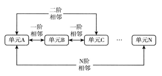
Figure 17.1: 高阶相邻一般用来分析空间影响效应的衰减过程。
18 空间面板数据模型
参考 姜磊 (2020, 1:6.3.4),五种空间面板模型
- 无固定效应的面板数据模型
- 空间固定效应的面板数据模型
- 时间固定效应的面板数据模型
- 空间和时间双固定效应的面板数据模型
- 随机效应的面板数据模型
18.1 空间固定效应
参考 姜磊 (2020, 1:6.2.2.1)
2000年后空间计量的关注从截面数据转移到面板数据,对于空间面板数据,类似于面板数据主要考虑个体效应(aka spatial specific effect)和时间效应,控制遗漏变量问题(GMM模型)(姜磊 2020, 1:263–64)
固定效应需要分为空间的和时间的。
\[ y_{i t}=X_{i t} \beta+\varepsilon_{i t} \]
变形后
\[ y_{i t}=\boldsymbol{X}_{i t} \boldsymbol{\beta}+\mu_{i}+\varepsilon_{i} \]
当\(\mu_{i}\)和自变量相关,那么就是固定效应; 当\(\mu_{i}\)和自变量无关,独立同分布,那么就是随机效应。
这一类个体效应, 如地理位置,也可以用地理权重矩阵完成,但只是用相邻关系决定; 如宗教信仰,也可以用文化距离权重矩阵完成,但只是用相邻关系决定。
18.2 时间固定效应
参考 姜磊 (2020, 1:6.2.1.2)
\[ y_{i t}=\boldsymbol{X}_{i t} \boldsymbol{\beta}+\gamma_{t}+\varepsilon_{i} \]
如对一个区域所有地区进行的政策。
当\(\gamma_{i}\)和自变量相关,那么就是固定效应; 当\(\gamma_{i}\)和自变量无关,独立同分布,那么就是随机效应。
18.3 双固定效应模型
参考 姜磊 (2020, 1:6.2.2)
也就是空间和时间两维度都包括固定效应的模型,也叫做 two way fixed effects。 常用的是 demean 法。
\[ \begin{aligned} &y_{i t}^{*}=y_{i t}-\frac{1}{T} \sum_{t=1}^{T} y_{i t}\\ &X_{i t}^{*}=X_{i t}-\frac{1}{T} \sum_{t=1}^{T} X_{i} \end{aligned} \]
\[ y_{i t}^{*}=\boldsymbol{X}_{i t}^{*} \boldsymbol{\beta}+\varepsilon_{i t}^{*} \]
然后采用 OLS 估计。
18.4 随机效应
参考 姜磊 (2020, 1:6.2.3)
\[ \left\{\begin{array}{l} y_{i t}=y_{i t}-(1-\theta) \frac{1}{T} \sum_{t=1}^{T} y_{i t} \\ X_{i t}^{*}=X_{i t}-(1-\theta) \frac{1}{T} \sum_{t=1}^{T} X_{i t} \end{array}\right. \]
如果\(\theta=0\)就是固定效应,因此对其进行LR检验,H_0为\(\theta=0\),拒绝的话,就是随机效应。
附录
参考文献
Anselin, Luc, Anil K. Bera, Raymond Florax, and Mann J. Yoon. 1993. “Simple Diagnostic Tests for Spatial Dependence.” Regional Science & Urban Economics 26 (1): 77–104.
Arbia, Giuseppe. 2014. A Primer for Spatial Econometrics: With Applications in R. 1st ed. Palgrave Texts in Econometrics. Palgrave Macmillan UK.
Baltagi, Badi H., Seuck Heun Song, Byoung Cheol Jung, and Won Koh. 2007. “Testing for Serial Correlation, Spatial Autocorrelation and Random Effects Using Panel Data.” Journal of Econometrics 140 (1): 5–51.
Franzese, Robert J., and Jude C. Hays. 2007. “Spatial Econometric Models of Cross-Sectional Interdependence in Political Science Panel and Time-Series-Cross-Section Data.” Political Analysis 15 (2): 140–64.
Kapoor, Mudit, Harry H. Kelejian, and Ingmar R. Prucha. 2007. “Panel Data Models with Spatially Correlated Error Components.” Journal of Econometrics 140 (1): 97–130.
Lee, Lung-fei, and Jihai Yu. 2010. “Estimation of Spatial Autoregressive Panel Data Models with Fixed Effects.” In.
———. 2012. “SPATIAL Panels: RANDOM Components Versus Fixed Effects*.” International Economic Review 53 (4): 1369–1412. https://doi.org/10.1111/j.1468-2354.2012.00724.x.
Millo, Giovanni. 2014. “Maximum Likelihood Estimation of Spatially and Serially Correlated Panels with Random Effects.” Computational Statistics & Data Analysis 71: 914–33.
———. 2017. “A Simple Randomization Test for Spatial Correlation in the Presence of Common Factors and Serial Correlation.” Regional Science & Urban Economics 66.
Mussa, Abeba, Uwaoma G. Nwaogu, and Susan Pozo. 2017. “Immigration and Housing: A Spatial Econometric Analysis.” Journal of Housing Economics 35: 13–25.
Mutl, Jan, and Michael Pfaffermayr. 2011. “The Hausman Test in a Cliff and Ord Panel Model.” Econometrics Journal 14 (1): 48–76.
Pesaran, M. Hashem. 2004. “General Diagnostic Tests for Cross Section Dependence in Panels.” Cambridge Working Papers in Economics 69 (7): 1240.
Sparks, Corey S. 2016. “Spatial Analysis Workshop - Code Examples - Social Science Consortium.” GitHub. 2016. http://htmlpreview.github.io/?https://github.com/coreysparks/Rcode/blob/e45d0147050cbe06b0dcdecc6a4ca8f07a91e522/Seminar_Code_2016.html.
Yang, Tse-Chuan, Aggie J. Noah, and Carla Shoff. 2015. “Exploring Geographic Variation in Us Mortality Rates Using a Spatial Durbin Approach.” Population, Space and Place 21 (1): 18–37. https://doi.org/10.1002/psp.1809.
姜磊. 2020. 应用空间计量经济学. 1st ed. Vol. 1. 1st Ser. 中国人民大学出版社.
杨攻研, and 刘洪钟. 2019. “贸易往来、选举周期与国家间政治关系-基于东亚地区的考证.” 国关国政外交学人. 2019. https://mp.weixin.qq.com/s/QASIg1JavV5Gi6iaWbiJ9w.
洪源, 陈丽, and 曹越. 2020. “地方竞争是否阻碍了地方政府债务绩效的提升?——理论框架及空间计量研究.” 金融研究 478 (4): 70–90.
王庆喜. 2014. 区域经济研究实用方法:基于ArcGIS.GeoDa和R的运用. 1st ed. Vol. 1. 1st Ser. 经济科学出版社.
王晴晴. 2019. “移民与住房:基于空间计量模型分析.” 好望角数据公社. 2019. https://mp.weixin.qq.com/s/5q-o1MK0l0bLmBUrVb12cA.
苏丹妮, 盛斌, and 邵朝对. 2019. “国内价值链、市场化程度与经济增长的溢出效应.” 世界经济 10 (August): 143–68.
董直庆, and 王辉. 2019. “城镇化、经济集聚与区域经济增长异质性——基于空间面板杜宾模型的经验证据.” 学术月刊. 2019. https://mp.weixin.qq.com/s/JyyELlfSoDRoXqRPHIDjUQ.