文本分析 学习笔记
2020-09-28
- 使用 RMarkdown 的
child参数,进行文档拼接。 - 这样拼接以后的笔记方便复习。
1 DTM Minimal Example
以下对 DTM (Document-Term Matrix) 进行举例。
- Due to bad loans, the bank agreed to pay the fines
- If you are late to pay off your loans to the bank, you will face fines
- A new restaurant opened in downtown
- There is a new restaurant that just opened on Warwick street
- How will you pay off the loans you will need for the restaurant you want opened?
如上是五个句子(Docs),进行分词后,产生词汇(Terms, bag of words),如下图。
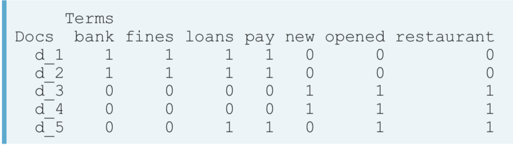
如果我们只考虑两种主题
- loan 贷款相关
- restaurant 餐饮相关
这里可以发现 d_5 算是有两种主题。
A dtm is a bag-of-words representation of text: the word order is lost. (Oleinikov 2019)
因此 dtm 是一个词包,忽略了词语的顺序,因此算是一种 naive 的模型,这就是 dtm 的定义了。
1.1 文档口径定义
Documents can be constructed in multiple way: they can be based on chapters in a novel, on paragraphs, or even on a sequence of several words. (Oleinikov 2019)
因此文档是可以自定义的。按照目前的短信需求,就是可以把一个用户的所有短信看成是一个文档。
Suppose a vandal has broken into your study and torn apart four of your books:
- Great Expectations by Charles Dickens
- The War of the Worlds by H.G. Wells
- Twenty Thousand Leagues Under the Sea by Jules Verne
- Pride and Prejudice by Jane Austen
This vandal has torn the books into individual chapters, and left them in one large pile. (Silge and Robinson 2019)
这和我目前处理的小说推荐器类似,直接 collapse 了。
2 NLP矩阵样本认识
参考 Ledolter (2013)
suppressMessages(library(tidyverse))
library(textir)
data(we8there) ## 6166 reviews and 2640 bigrams
dim(we8thereCounts)
## [1] 6166 2640## [1] "dgCMatrix"
## attr(,"package")
## [1] "Matrix"## 6 x 6 sparse Matrix of class "dgCMatrix"
## Terms
## Docs veri good go back dine room dine experi great food food great
## 1 . . . . . .
## 2 . . . . . .
## 5 . . . . . .
## 11 . . . . . .
## 12 . . . . . .
## 13 . . . . . .这是一个稀疏矩阵,数字衡量发生频率。 这里显示有 6166 个评论,一共形成了 2640 个词汇。
## [1] "veri good"   "go back"     "dine room"   "dine experi" "great food"
## [6] "food great"## [1] 2640## [1] "1" "2" "5" "11" "12" "13"## [1] 6166## [1] 6166 5选取第12号样本进行样本认识。
我们知道了we8thereCounts的 class,先转换成 matrix 进行分析。
##   veri good     go back   dine room dine experi  great food
##           0           0           0           0           0
这是第12个样本,前五个词的的发生频率。他们是从高到低排列的,证明如下。
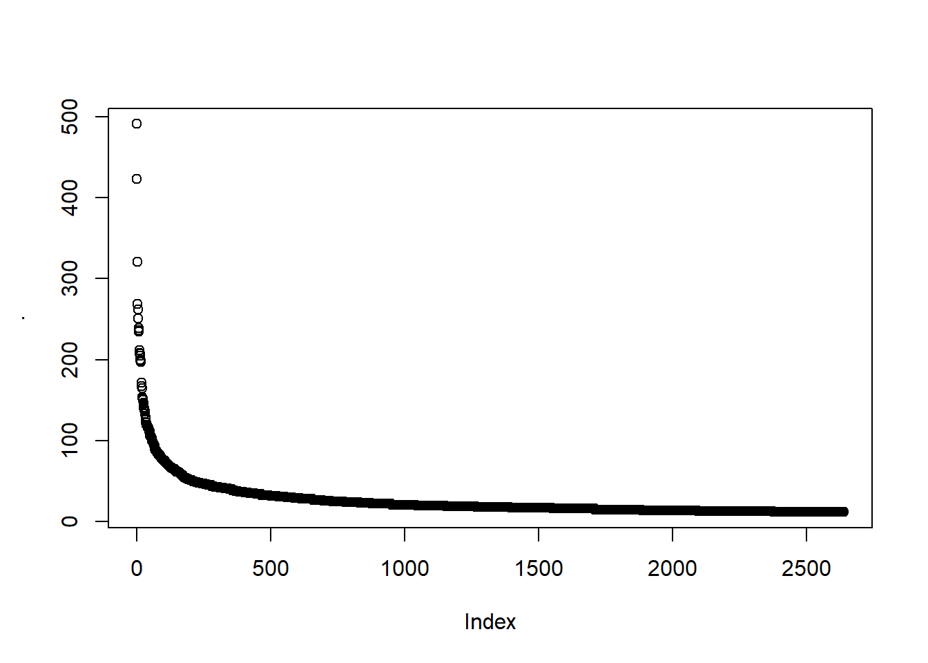
因此这些都是重要的词,不是每个词汇都会被计入,只计入重要的。
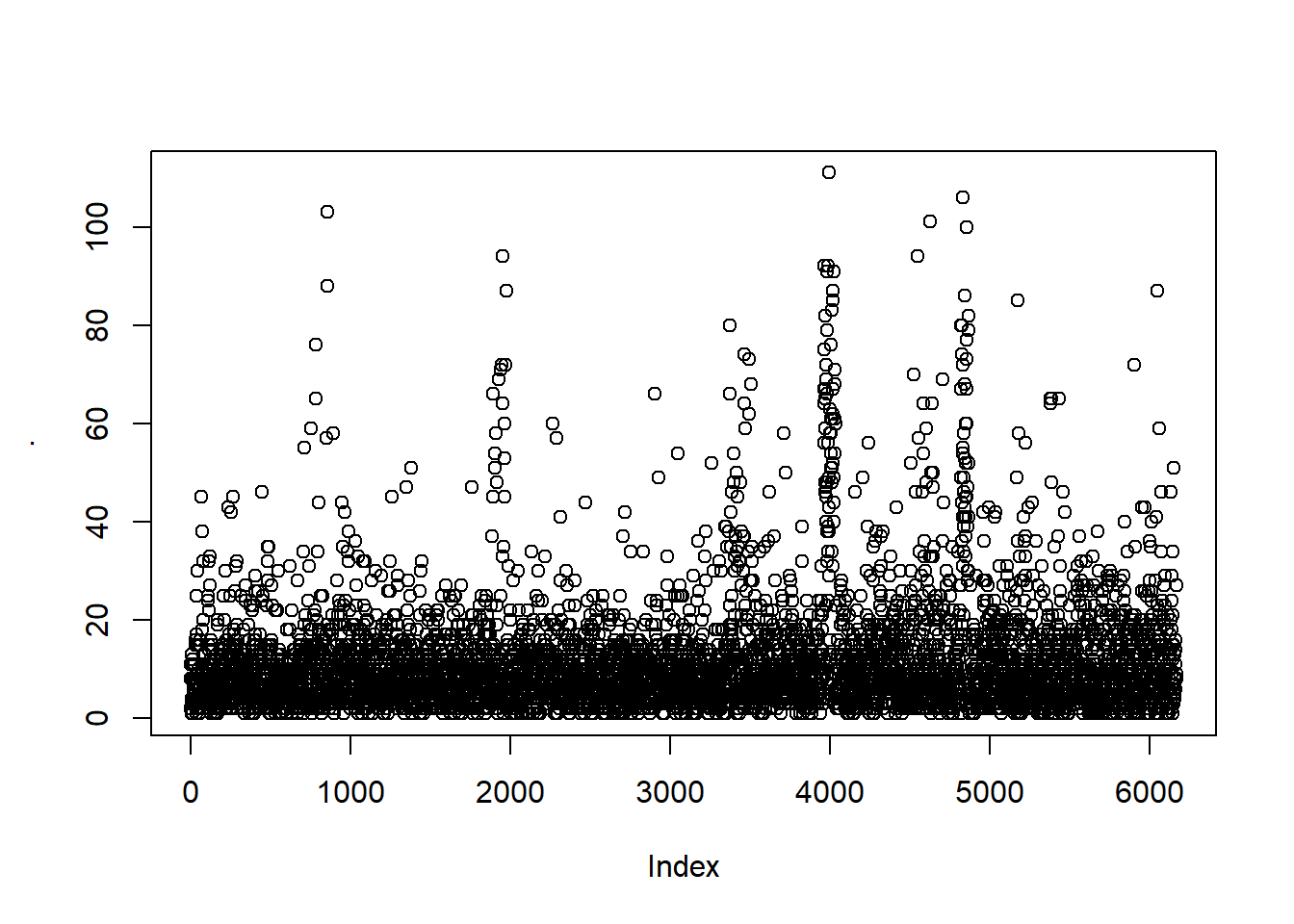
这可以看到大部分的评论长度集中在10个 biggrams 左右。
## [1] 13在一个样本一个词出现最多的情况是13次。
目前来看,只要转换成这样一个矩阵,那么就可以进行训练了,其次就是要各样本每个词的频数,转换成经典的分类模型问题。
3 停用词
stopwords 其实就是一个 vector,这里已经有总结的很好的,参考 github,其中就有中文的停用词。 测试例子,参考 Github Pages
参考 Ledolter (2013)
The next step is to search the text documents for a list of stop words containing irrelevant words marked for removal. If, and, but, who, what, the, they, their, a, or, and so on are examples of stop words that need to be removed. But one needs to be careful because one person’s stop word is another’s key term.
stop words 就是一些词不需要进入模型的,进而删除。
Also, one usually removes words that are extremely rare. …… A reasonable rule removes words with relative frequencies below 0.5%.
一般有三种方式
- 根据业务经验,比如“的”
- 比例太小,比如小于 0.5% 以下
- 按照tf-idf打分
3.1 用停用词分词
参考 Shrivarsheni (2020)

Figure 3.1: 停用词的两种用法,一种是保持在分词时,不将停用词分开;一种是不将停用词分开且删除停用词,这一步和正则化不同,正则化假设在这里要删除’天真’,会直接把’天真’删除,破坏分词’今天’和’真好’。
How to tokenize text with stopwords as delimiters? Difficulty Level : L2 Q. Tokenize the given text with stop words (“is”,”the”,”was”) as delimiters. Tokenizing this way identifies meaningful phrases. Sometimes, useful for topic modeling
# Input :
text = "Walter was feeling anxious. He was diagnosed today. He probably is the best person I know."
text
# Expected Output :
['Walter',
 'feeling anxious',
 'He',
 'diagnosed today',
 'He probably',
 'best person I know']
# Solution
text = "Walter was feeling anxious. He was diagnosed today. He probably is the best person I know."
stop_words_and_delims = ['was', 'is', 'the', '.', ',', '-', '!', '?']
for r in stop_words_and_delims:
text = text.replace(r, 'DELIM')
words = [t.strip() for t in text.split('DELIM')]
words_filtered = list(filter(lambda a: a not in [''], words))
words_filtered## ['Walter', 'feeling anxious', 'He', 'diagnosed today', 'He probably', 'best person I know']这里总结一下,
- 统一停用词
replace(r, 'DELIM') - 用停用词切分
.split('DELIM')] - 删除多余空格
.strip() - 删除
'',filter(lambda a: a not in [''], words),防止len([]) is None的情况。
这是停用词的用法。
jieba.cut也可以但是和其他 textrank 不兼容。
3.2 SQL 方式剔除停用词
参考 Oleinikov (2019)
# Create the document-term matrix with stop words removed
dtm <- corpus %>%
  unnest_tokens(output=word, input=text) %>%
  anti_join(stop_words) %>%
  dplyr::count(id, word) %>%
  cast_dtm(document=id, term=word, value=n)

# Display the matrix
as.matrix(dtm)
## Terms
## Docs bad due loans bank late pay downtown restaurant street warwick
## 1 1 1 1 0 0 0 0 0 0 0
## 2 0 0 1 1 1 1 0 0 0 0
## 3 0 0 0 0 0 0 1 1 0 0
## 4 0 0 0 0 0 0 0 1 1 1
## 5 0 0 1 0 0 1 0 1 0 0参考 DataCamp
主要使用函数anti_join完成,非常有关系库代码的含义。
会发现加入停用词后会改变,矩阵的空间结构,从而改变整个概率计算,因此是非常有意义的。
4 云图
参考 Oleinikov (2019)
# Generate the counts of words in the corpus
word_frequencies <- corpus %>%
  unnest_tokens(input=text, output=word) %>%
  dplyr::count(word)

# Create a wordcloud
wordcloud::wordcloud(words=word_frequencies$word,
          freq=word_frequencies$n,
          min.freq=1,
          max.words=10,
          colors=wesanderson::wes_palette("Royal1"),
          random.order=FALSE,
          random.color=FALSE)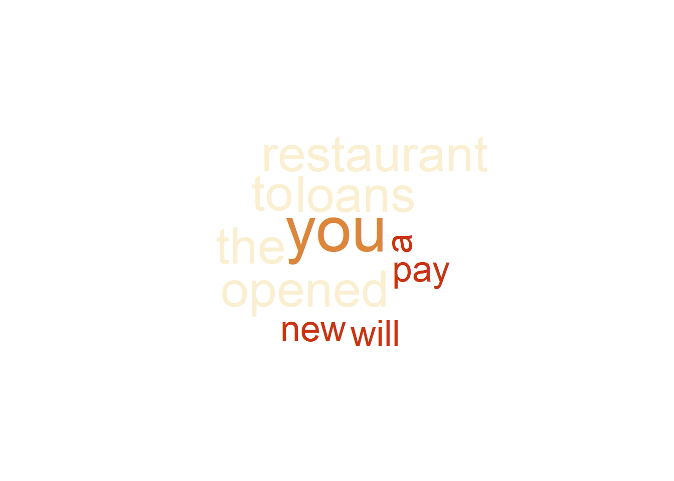
min.freq=1频率至少多少放入max.words=10展示 top 几colors可以加入调色盘
5 tf-idf
参考 Ledolter (2013)
tf-idf (term frequency/inverse document frequency) score
\[\text{tf-idf} = f_{ij} \times \log(\frac{n}{d_j})\]
Consider a document containing 10,000 words wherein the word donkey appears 300 times. Following the earlier definition, the term frequency (tf) for donkey is (300/10, 000) = 0.03. Now, assume we have 1,000 documents and donkey appears in 10 of these. Then, its inverse document frequency (idf) is calculated as log (1000/10) = 2. The tf-idf score is the product of these quantities: 0.03 × 2 = 0.06
假设一个文档有1万个字,其中含有donkey这个词有300词,
那么
\[\text{tf} = 300/10000 = 0.03\]
假设现在有1000个文档,其中有10个文档含有 doukey 这个文字,那么
\[\text{idf} = \log(1000/10) = 2\]
因此得分为
\[\text{tf-idf} = 0.03 \times 2 = 0.06\]
Several other preprocessing steps can be used to get a meaningful list of words and their counts (frequencies). Words can be single words, or bigrams of words. Bigrams are groups of two adjacent words, and such bigrams are commonly used as the basis for the statistical analysis of text. Bigrams can be extended to trigrams (three adjacent words) and, more general, n-grams, which are sequences of n adjacent words.
同时我们发现这样的计算也有问题,就是不考虑词组,因此出现了 n-grams 是专门加入了词组考量的。
5.1 tf 的直观理解
One measure of how important a word may be is its term frequency (tf), how frequently a word occurs in a document
这是 term frequency 的定义,非常直观。
5.2 idf 引入的原因
There are words in a document, however, that occur many times but may not be important; in English, these are probably words like “the”, “is”, “of”, and so forth.
这类词,可以用 stopwords 的方式完成。
Another approach is to look at a term’s inverse document frequency (idf), which decreases the weight for commonly used words and increases the weight for words that are not used very much in a collection of documents. This can be combined with term frequency to calculate a term’s tf-idf (the two quantities multiplied together), the frequency of a term adjusted for how rarely it is use.
因此 idf 就是一个 stopwords 更好的替代品。
\[\text{idf}(\text{term}) = \log (\frac{n_{\text{documents}}}{n_{\text{documents containing term}}})\]
这里做了倒数处理。
Calculating tf-idf attempts to find the words that are important (i.e., common) in a text, but not too common.
tf-idf 的直观理解。
- t - term
- d - document
library(dplyr)
library(janeaustenr)
library(tidytext)

book_words <- austen_books() %>%
  unnest_tokens(word, text) %>%
  dplyr::count(book, word, sort = TRUE)

total_words <- book_words %>%
  dplyr::group_by(book) %>%
  dplyr::summarize(total = sum(n))

book_words <- left_join(book_words, total_words)

book_wordsHere we see all proper nouns, names that are in fact important in these novels. None of them occur in all of novels, and they are important, characteristic words for each text within the corpus of Jane Austen’s novels.
都是一些人名、名词。
5.3 验证函数 bind_tf_idf
5.4 验证 tf 是否计算对
完全一致。
5.5 验证 idf 是否计算对
df_matrix <-
    book_words %>%
    ungroup() %>%
    group_by(word) %>%
    dplyr::count() %>%
    dplyr::rename(n_document_included = n)
book_words %>%
    ungroup() %>%
    mutate(n_document = n_distinct(book)) %>%
    ungroup() %>%
    left_join(df_matrix) %>%
    mutate(idf_var = log(n_document/n_document_included)) %>%
    ungroup() %>%
    summarise(mean(idf != idf_var))
5.6 tf-idf 的应用场景
Using term frequency and inverse document frequency allows us to find words that are characteristic for one document within a collection of documents, whether that document is a novel or physics text or webpage.
tf-idf 可以查看 一堆文档中,最重要的词汇是什么, 这些文档可以是网页、科技文档、小说。
6 使用 Xgboost 进行简单预测
参考 Ledolter (2013) 和 参考NLP矩阵样本认识,接下来做一些简单的预测。
suppressMessages(library(tidyverse))
library(textir)
library(xgboost)
library(knitr)
library(here)
data(we8there) ## 6166 reviews and 2640 bigrams
方便的是,x 这个矩阵已经准备好了,我们做训练。
overall <- we8thereRatings$Overall
library(caret)
idx <- caret::createDataPartition(y = overall, times = 1, p = 0.8, list = F)
y_train <- overall[ idx]
y_test  <- overall[-idx]
length(y_train) + length(y_test) == length(overall)
x_train <- as.matrix(we8thereCounts)[ idx,]
x_test <- as.matrix(we8thereCounts)[-idx,]library(xgboost)
dtrain <- xgb.DMatrix(x_train, label = y_train)
dtest <- xgb.DMatrix(x_test, label = y_test)
watchlist <- list(eval = dtest, train = dtrain)mod <- xgb.train(
data = dtrain,
eta = 0.1,
max_depth = 3,
nround=20,
subsample = 0.5,
colsample_bytree = 0.5,
seed = 1,
objective = 'count:poisson',
# objective = "multi:softmax",
# num_class = 6,
watchlist = watchlist,
nthread = 3
)data_frame(
yhat = mod %>% predict(dtest),
y = y_test
) %>%
ggplot(aes(x = as.factor(y_test), y = yhat)) +
geom_jitter()
ggsave("figure/count-poisson-perf.png")
# ggsave("figure/multi-softmax-perf.png")测试 count:poisson 效果不佳。

测试 multi:softmax 效果。

7 主题模型
- 使用 RMarkdown 的
child参数,进行文档拼接。 - 这样拼接以后的笔记方便复习。
- 相关问题提交到 Issue
8 LDA summary
参考 https://www.cnblogs.com/pinard/p/6831308.html
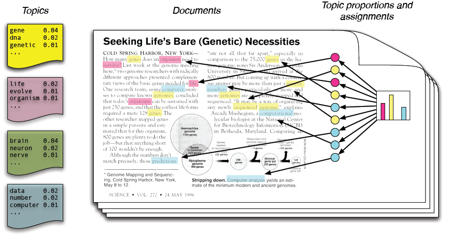
LDA,全称为 Latent Dirichlet Allocation 狄利克雷(德国)。 这是基于贝叶斯的模型。 先验分布 + 经验/数据 = 后验分布。 然后后验分布和先验分布是同一种分布,因此是可以循环的共轭分布。 这里采用二分类的 beta 分布,LDA 就是多分类版本的 beta 分布。 因此以 beta 分布举例即可。 我们假设 100个好人,100个坏人,这是我们的先验分布,通过数据和经验,我们得到2个好人和1个坏人,现在后验分布为 102个好人和101个坏人。然后依次循环。
在主题模型中,
\[ \beta_{i j}=\frac{C_{i j}^{W T}+\eta}{\sum_{k=1}^{W} C_{k j}^{W T}+W \eta} \quad \theta_{d j}=\frac{C_{d j}^{D T}+\alpha}{\sum_{k=1}^{T} C_{d k}^{D T}+T \alpha} \]
- 文档-主题的先验分布为 theta 分布,对应超参数 alpha,需要先赋值,越大,主题差异越
大小,主题分越均匀,当 alpha 越大,\(\frac{C_{d j}^{D T}+\alpha}{\sum_{k=1}^{T} C_{d k}^{D T}+T \alpha} \to \frac{\alpha}{T \alpha}\)。alpha 是 K 维度向量,K 是先验的,主题数量。统计意义是 24% words in doc1 属于 topic1。 - 主题-词汇的先验分布为 beta 分布,对应超参数 eta,需要先赋值,越大,这个主题的有更多的词汇,当 eta 越大,\(\frac{C_{i j}^{W T}+\eta}{\sum_{k=1}^{W} C_{k j}^{W T}+W \eta} \to \frac{\eta}{W \eta}\)。beta 是 V 维度向量,V 是词语表大小。
LDA 的输入是 doc-term 的分布,这个也是先验的,可以用词频、也可以用 tf-idf。
最大化 log-likelihood 得到后验分布。
主题重叠,同样高频的关键词可以出现在两个主题上。
Perplexity 是 Held out 思想,alpha、beta 确定以后,可以预测到一个测试集上。 比如说主题数为3和4的两种情况,对应每个主题的 P概率/ [NO. tokens] 越平均,越不好。 目标是最大概率,因此 Perplexity 是取反了,越小越好。
9 Blei, Ng, and Jordan (2003)
LDA(Blei, Ng, and Jordan 2003) 是的 Andrew Ng 二作,Michael I. Jordan 是三作,一作 Blei 后续产出了很多 TM 的变形。
In this paper we consider the problem of modeling text corpora and other collections of discrete data. The goal is to find short descriptions of the members of a collection that enable efficient processing of large collections while preserving the essential statistical relationships that are useful for basic tasks such as classification, novelty detection, summarization, and similarity and relevance judgments.
可以帮助新词发现。
The end result is a term-by-document matrix X whose columns contain the tf-idf values for each of the documents in the corpus. Thus the tf-idf scheme reduces documents of arbitrary length to fixed-length lists of numbers.
主题模型之前是tf-idf,当然也有各种弱点。
the approach also provides a rela- tively small amount of reduction in description length and reveals little in the way of inter- or intra- document statistical structure.
从描述性统计上讲,tf-idf 的 terms 太多,没有怎么做降维;并且没有把文档内和外的结构进行展示。
试想一下 LDA,我们可以知道一个文档的主题分布,可以文档间主题差异。
most notably latent semantic indexing (LSI) (Deerwester et al., 1990). LSI uses a singular value decomposition of the X matrix to identify a linear subspace in the space of tf-idf features that captures most of the variance in the collection.
LSI 是 tf-idf 的降维。
Furthermore, Deerwester et al. argue that the derived features of LSI, which are linear combinations of the original tf-idf features, can capture some aspects of basic linguistic notions such as synonymy and polysemy.
- LSI 在 tf-idf 的基础上,还包含了同义词等的提取?可以理解一下,找一下论文。
Given a generative model of text, however, it is not clear why one should adopt the LSI methodology—one can attempt to proceed more directly, fitting the model to data using maximum likelihood or Bayesian methods.
Blei, Ng, and Jordan (2003) 认为 LSI 不够直接,借助于 tf-idf,可以直接对 text data 做ML,或者贝叶斯方法。
A significant step forward in this regard was made by Hofmann (1999), who presented the probabilistic LSI (pLSI) model, also known as the aspect model, as an alternative to LSI. The pLSI approach, which we describe in detail in Section 4.3, models each word in a document as a sample from a mixture model, where the mixture components are multinomial random variables that can be viewed as representations of “topics.” Thus each word is generated from a single topic, and different words in a document may be generated from different topics. Each document is represented as a list of mixing proportions for these mixture components and thereby reduced to a probability distribution on a fixed set of topics. This distribution is the “reduced description” associated with the document.
pPSI 和 LDA 在词汇上的处理方式很类似。
While Hofmann’s work is a useful step toward probabilistic modeling of text, it is incomplete in that it provides no probabilistic model at the level of documents. In pLSI, each document is represented as a list of numbers (the mixing proportions for topics), and there is no generative probabilistic model for these numbers. This leads to several problems: (1) the number of parame- ters in the model grows linearly with the size of the corpus, which leads to serious problems with overfitting, and (2) it is not clear how to assign probability to a document outside of the training set.
不是特别懂,但是不方便文档在测试集上预测。
9.1 Notation and terminology
Indeed, in Section 7.3, we present experimental results in the collaborative filtering domain.
CF 中在原论文的提到,可以使用 LDA。
后面可以关注 Griffiths and Steyvers (2004) 在吉普斯采样上的优化。
10 Griffiths and Steyvers (2004)
Our method discovers a set of topics expressed by documents, providing quantitative measures that can be used to identify the content of those documents, track changes in content over time, and express the similarity between documents.
We use these topics to illustrate the relationships between different scientific disciplines, assessing trends and ‘‘hot topics’’ by analyzing topic dynamics and using the assignments of words to topics to highlight the semantic content of documents.
似乎 Griffiths and Steyvers (2004) 已经考虑时间在主题模型上面的使用了。
\[ P\left(w_{i}\right)=\sum_{j=1}^{T} P\left(w_{i} \mid z_{i}=j\right) P\left(z_{i}=j\right) \]
where \(z_{i}\) is a latent variable indicating the topic from which the ith word was drawn and \(P\left(w_{i} \mid z_{i}=j\right)\) is the probability of the word \(w_{i}\) under the \(j\) th topic. \(P\left(z_{i}=j\right)\) gives the probability of choosing a word from topics \(j\) in the current document, which will vary across different documents.
Intuitively, \(P(w \mid z)\) indicates which words are important to a topic, whereas \(P(z)\) is the prevalence of those topics within a document.
- \(P\left(w_{i}\right)\) 衡量在 word i 在当前文档的里面的无条件概率
- \(P\left(z_{i}=j\right)\) 衡量 word i 在当前文档的里面多分类主题上的无条件概率
- \(P\left(w_{i} \mid z_{i}=j\right)\) 衡量 word i 在当前文档的里面多分类主题 j 上的条件概率
For example, in a journal that published only articles in mathematics or neuroscience, we could express the probability distribution over words with two topics, one relating to mathematics and the other relating to neuroscience. The content of the topics would be reflected in \(P(w \mid z) ;\) the “mathematics” topic would give high probability to words like theory, space, or problem, whereas the “neuroscience” topic would give high probability to words like synaptic, neurons, and hippocampal.
\(P\left(w_{i} \mid z_{i}=j\right)\) 主要看某一个主题里面的关键词分布。
Whether a particular document concerns neuroscience, mathematics, or computational neuroscience would depend on its distribution over topics, \(P(z),\) which determines how these topics are mixed together in forming documents. The fact that multiple topics can be responsible for the words occurring in a single document discriminates this model from a standard Bayesian classifier, in which it is assumed that all the words in the document come from a single class. The “soft classification” provided by this model, in which each document is characterized in terms of the contributions of multiple topics, has applications in many domains other than text (7) .
\(P\left(z_{i}=j\right)\) 主要看文档里面主题的分布。
Viewing documents as mixtures of probabilistic topics makes it possible to formulate the problem of discovering the set of topics that are used in a collection of documents. Given \(D\) documents containing \(T\) topics expressed over \(W\) unique words,
LDA 三个最主要的参数。
we can represent \(P(w \mid z)\) with a set of \(T\) multinomial distributions \(\phi\) over the \(W\) words, such that \(P(w \mid z=j)=\phi_{w}^{(j)},\) and \(P(z)\) with a set of \(D\) multinomial distributions \(\theta\) over the \(T\) topics, such that for a word in document \(d, P(z=j)=\theta_{j}^{(d)} .\) To discover the set of topics used in a corpus \(\mathbf{w}=\left\{w_{1}, w_{2}, \ldots, w_{n}\right\},\) where each \(w_{i}\) belongs to some document \(d_{i},\) we want to obtain an estimate of \(\phi\) that gives high probability to the words that appear in the corpus. One strategy for obtaining such an estimate is to simply attempt to maximize \(P(\mathbf{w} \mid \phi, \theta),\) following from Eq. \(\mathbf{1}\) directly by using the Expectation-Maximization (8) algorithm to find maximum likelihood estimates of \(\phi\) and \(\theta(2,3) .\) However, this approach is susceptible to problems involving local maxima and is slow to converge \((1,2),\) encouraging the development of models that make assumptions about the source of \(\theta .\)
这里的 \(\phi\) 其实对应的是 \(\gamma\) 分布,是主题-词的分布。
所以最后公式变成
\[ P\left(w_{i} \mid z_{i}=j\right) = P\left(w_{i}\right)=\sum_{j=1}^{T} P\left(w_{i} \mid z_{i}=j\right) P\left(z_{i}=j\right) \]
10.1 Conclusion

Figure 10.1: 方便可视化主题模型的效果。
11 Phan, Nguyen, and Horiguchi (2008)
参考 1367497.1367510.pdf
The main motivation of this work is that many classification tasks working with short segments of text & Web, such as search snippets, forum & chat messages, blog & news feeds, product reviews, and book & movie summaries, fail to achieve high accuracy due to the data sparseness.
短文本的主要问题是稀疏。
The underlying idea of the framework is that for each classification task, we collect a very large external data collection called “universal dataset”, and then build a classification model on both a small set of labeled training data and a rich set of hidden topics discovered from that data collection. The framework is mainly based on recent successful latent topic analysis models, such as pLSA [22] and LDA [8], and powerful machine learning methods like maximum entropy and SVMs. The main advantages of the framework include the following points:
- LDA 在这个地方扮演了什么角色?
Reducing data sparseness: while uncommon words preserve the distinctiveness among training examples, hidden topics do make those examples more related than the original. Including hidden topics in training data helps both reduce the sparseness and make the data more topic-focused.
当把数据稀疏问题解决后,那么数据会更加的主题上聚合。
Flexible semi-supervised learning: this framework can also be seen as a semi-supervised method because it can utilize unlabeled data to improve the classifier. However, unlike traditional semi-supervised learning algorithms [11, 29], the universal data and the training/test data are not required to have the same format. In addition, once estimated, a topic model can be applied to more than one classification problems provided that they are consistent
- 其实需要看懂框架才能理解这些优点

Figure 11.1: 整体还是一个分类模型。
12 张志飞, 苗夺谦, and 高灿 (2013)
参考 张志飞, 苗夺谦, and 高灿 (2013) review 一遍 LDA。
LDA 主题模型由 Blei 等提出,是一个“文本一主题一 词”的三层贝叶斯产生式模型,每篇文本表示为主题的混合 分布,而每个主题则是词上的概率分布。 最初的模型只对文 本一主题概率分布引入一个超参数使其服从 Dirichlet 分布, 随后 Griffiths 等 对主题一词概率分布也引入一个超参数使 其服从 Dirichlet 分布。 该模型用图 1 表示,各符号的含义如 表 1 所示。
所以严格来说,LDA 是 Blei 和 Griffiths 一起提出的。

Figure 12.1: 图中的超参数 beta 一般也是 eta 符号表示,表示词-主题的多分类分布。目前这个示意图一目了然,两个超参数 alpha 和 beta 一起作用于 theta 和 gamma 分布,对词在主题上的分布进行作用。
两个超参数一般设置为 \(\alpha=50 / T, \beta=0.01\)。
LDA 模 型的参数个数只与主题数和词数有关,参数估计是计算出文 本一主题概率分布以及主题一词概率分布,即 \(\boldsymbol{\theta}\) 和 \(\boldsymbol{\varphi}\) 。通过对 变量 z 进行 Gibbs 采样间接估算 \(\boldsymbol{\theta}\) 和 \(\boldsymbol{\varphi}\) :
\[ \begin{aligned} \theta_{m s} &=\frac{n_{m}^{(s)}+\alpha}{\sum_{j=1}^{T} n_{m}^{(j)}+T \alpha} \\ \varphi_{s k} &=\frac{n_{s}^{(k)}+\beta}{\sum_{i=1}^{N} n_{s}^{(i)}+N \beta} \end{aligned} \]
其中:n_m 表示文本 \(d_{m}\) 中赋予主题 \(j\) 的词的总数, \(n_{s}^{(i)}\) 表示词 \(v_{i}\) 被赋子主题 \(s\) 的总次数。
因此一般来说,\(\beta=0.01\)就是偏小了,会让整个主题里面的关键词很少。
13 \(\eta\) rate schedule

Figure 13.1: LDA的分布从\(\beta\)分布中衍生出来,是多分类的,其中\(\eta\)是控制如图 Gibbs 采样中,后验分布被先验分布更新的参数,这个参数是用于正则化的,但是可以每一次迭代都不一样。因此可以产生两种策略,一种是先大\(\eta\)后小\(\eta\),一种是先小\(\eta\)后大\(\eta\)。其中大\(\eta\)正则化强,因此每个主题分之间更加’均匀’,反正差异大。
14 build ngram
rely on the bag-of-words assumption. They thus lose the semantic ordering of the words inherent in the text which can give an extra leverage to the computational model. (Jameel and Lam 2013)
ngram
but also generates topi- cal n-gram words leading to more interpretable latent topics in the family of the nonparametric topic models. (Jameel and Lam 2013)
提高可读性。
14.1 bigram
参考 Shrivarsheni (2020)
How to create bigrams using Gensim’s Phraser ? Difficulty Level : L3 Q. Create bigrams from the given texts using Gensim library’s Phrases
# Input :
sdocuments = ["the mayor of new york was there", "new york mayor was present"]
sdocuments
# Desired Output:
## ['the mayor of new york was there', 'new york mayor was present']## [['the', 'mayor', 'of', 'new york', 'was', 'there'], ['new york', 'mayor', 'was', 'present']]## [['the', 'mayor', 'of', 'new', 'york', 'was', 'there'], ['new', 'york', 'mayor', 'was', 'present']]空格切分
# Show Solution
# Import Phraser from gensim
from gensim.models import Phrases
from gensim.models.phrases import Phraser

# Creating bigram phraser
bigram = Phrases(sentence_stream, min_count=1, threshold=2, delimiter=b' ')
bigram_phraser = Phraser(bigram)

for sent in sentence_stream:
    tokens_ = bigram_phraser[sent]
    print(tokens_)
## ['the', 'mayor', 'of', 'new york', 'was', 'there']
## ['new york', 'mayor', 'was', 'present']'new york'就一起出现了,同时减少了new和york的出现。
14.2 ngram
参考 Prabhakaran (2020) 就是一直嵌套。
# corpus = pd.Series({'text':text}).apply(lambda x: jieba_cut(x, stopwords))
corpus = text.apply(lambda x: jieba_cut(x, stopwords))
Building prefix dict from the default dictionary ...
Loading model from cache C:\Users\LIJIAX~1\AppData\Local\Temp\jieba.cache
Loading model cost 1.206 seconds.
Prefix dict has been built succesfully.bigram = Phrases(corpus, min_count=10, threshold=100, delimiter=b'-')
trigram = Phrases(bigram[corpus], min_count=10, threshold=100, delimiter=b'-')
quadgram = Phrases(trigram[corpus], min_count=10, threshold=100, delimiter=b'-')
bigram_phraser = Phraser(bigram)
trigram_phraser = Phraser(trigram)
quadgram = Phraser(quadgram)
corpus = [quadgram[trigram[bigram_phraser[sent]] ] for sent in corpus]参考 https://stackoverflow.com/a/43542876/8625228
from nltk.util import ngrams

sdocuments = ["the mayor of new york was there", "new york mayor was present"]

corpus = []
for doc_i in sdocuments:

    corpus_i = doc_i.strip().split(' ')

    corpus_output_i = ["-".join(i) for i in ngrams(corpus_i,3)]
    # join make the output in one scalar instead of tuple.
    corpus.append(corpus_output_i)

from pprint import pprint

pprint(sdocuments)
## ['the mayor of new york was there', 'new york mayor was present']## [['the-mayor-of',
## 'mayor-of-new',
## 'of-new-york',
## 'new-york-was',
## 'york-was-there'],
## ['new-york-mayor', 'york-mayor-was', 'mayor-was-present']]14.3 Paper Review
参考 Mikolov et al. (2013)
The bigrams with score above the chosen threshold are then used as phrases. Typically, we run 2-4 passes over the training data with decreasing threshold value,
\[\operatorname{score}\left(w_{i}, w_{j}\right)=\frac{\operatorname{count}\left(w_{i} w_{j}\right)-\delta}{\operatorname{count}\left(w_{i}\right) \times \operatorname{count}\left(w_{j}\right)}\]
threshold 来源。
allow- ing longer phrases that consists of several words to be formed.
threshold 越小,phrases 越多
Phrase Skip-Gram Results
原来对词向量训练也有用。
We successfully trained models on several orders of magnitude more data than the previously pub- lished models, thanks to the computationally efficient model architecture. This results in a great improvement in the quality of the learned word and phrase representations, especially for the rare entities. We also found that the subsampling of the frequent words results in both faster training and significantly better representations of uncommon words. Another contribution of our paper is the Negative sampling algorithm, which is an extremely simple training method that learns accurate representations especially for frequent words.
- 所以 threshold 是大是小好?没有找到。
The choice of the training algorithm and the hyper-parameter selection is a task specific decision, as we found that different problems have different optimal hyperparameter configurations. In our experiments, the most crucial decisions that affect the performance are the choice of the model architecture, the size of the vectors, the subsampling rate, and the size of the training window.
滑动窗口做样本。
Another approach for learning representations of phrases presented in this paper is to simply represent the phrases with a single token. Combination of these two approaches gives a powerful yet simple way how to represent longer pieces of text, while hav- ing minimal computational complexity.
这个简单的方法,效果还不错
14.4 nltk.util.ngram bug
5-gram 的情况是没有主题可以聚合出来,因为每一个关键词都是唯一的,所以连续n个词,都要看看唯一值占比。 数据量有200多万个文本,因此有偏的估计应该是不存在的。
模型整体来讲是做挂了。我用的是 5gram 做的,滑动窗口为5,取词方式如下。
 ['aaa-bb-c-dd-ee',
  'bb-c-dd-ee-dd',
  'c-dd-ee-dd-f',
  'dd-ee-dd-f-gg',
  'ee-dd-f-gg-hh',
  'dd-f-gg-hh-i'],
有一个处理没有做,就是小于5的,因为少于5,所以变成空了,这是预处理的时候,没有注意的。
但是>=5gram 全部滑动为5个词的样本;<=5gram再换一个方式比如单个关键词切一个词,也很奇怪,所以直接否了这个方案了。
严格来看,n-gram 应该还是一个 topic model 内部应该解决的事情, 不应该放到 corpus 直接粗暴的完成。 例如考虑 threshold 改成负数?
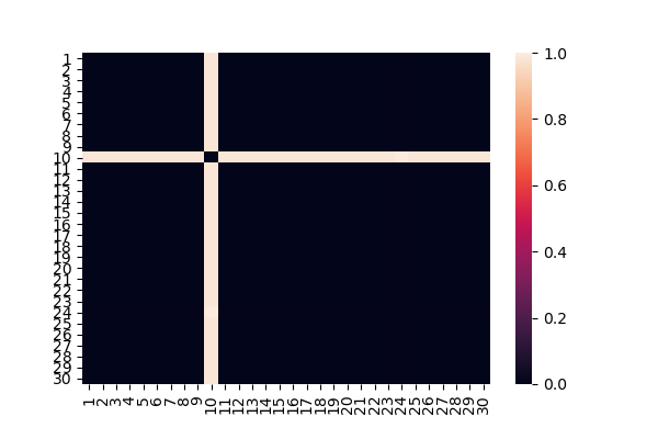
Figure 14.1: 因为主题对于所有的关键词权重为0,因此就是一个常数,常数和常数之间的相关性就为0了。
分析原因是因为生成词都是唯一的,在整个文档里面只出现了几次,因此没有大量的共现想象,因此无法被抽取为关键词,具体复现代码如下。
15 Gibbs Samping
This is essentially a clustering problem - can think of both words and documents as being clustered.(Clark and Gales 2013)
LDA 的初衷就是为了拿到词和文档的两种聚类。
参考 Liu (2015)
rawdocs <- c(
    "eat turkey on turkey day holiday",
    "i like to eat cake on holiday",
    "turkey trot race on thanksgiving holiday",
    "snail race the turtle",
    "time travel space race",
    "movie on thanksgiving",
    "movie at air and space museum is cool movie",
    "aspiring movie star"
)
docs <- strsplit(rawdocs, split = " ")
docs %>% head(2)
## [[1]]
## [1] "eat" "turkey" "on" "turkey" "day" "holiday"
##
## [[2]]
## [1] "i" "like" "to" "eat" "cake" "on" "holiday"## [1] "eat" "turkey" "on" "day" "holiday" "i"## [1] 8## [[1]]
## [1] 1 2 3 2 4 5
##
## [[2]]
## [1] 6 7 8 1 9 3 5
##
## [[3]]
## [1] 2 10 11 3 12 5
##
## [[4]]
## [1] 13 11 14 15
##
## [[5]]
## [1] 16 17 18 11
##
## [[6]]
## [1] 19 3 12
##
## [[7]]
## [1] 19 20 21 22 18 23 24 25 19
##
## [[8]]
## [1] 26 19 27完成匹配。
为了简单,假设主题数为 2。
# cluster number
K <- 2

# initialize count matrices
# @wt : word-topic matrix
wt <- matrix( 0, K, length(vocab) )
colnames(wt) <- vocab
wt
## eat turkey on day holiday i like to cake trot race thanksgiving snail the
## [1,] 0 0 0 0 0 0 0 0 0 0 0 0 0 0
## [2,] 0 0 0 0 0 0 0 0 0 0 0 0 0 0
## turtle time travel space movie at air and museum is cool aspiring star
## [1,] 0 0 0 0 0 0 0 0 0 0 0 0 0
## [2,] 0 0 0 0 0 0 0 0 0 0 0 0 0# @ta : topic assignment list
ta <- lapply( docs, function(x) rep( 0, length(x) ) )
names(ta) <- paste0( "doc", 1:length(docs) )
ta## $doc1
## [1] 0 0 0 0 0 0
##
## $doc2
## [1] 0 0 0 0 0 0 0
##
## $doc3
## [1] 0 0 0 0 0 0
##
## $doc4
## [1] 0 0 0 0
##
## $doc5
## [1] 0 0 0 0
##
## $doc6
## [1] 0 0 0
##
## $doc7
## [1] 0 0 0 0 0 0 0 0 0
##
## $doc8
## [1] 0 0 0# @dt : counts correspond to the number of words assigned to each topic for each document
dt <- matrix( 0, length(docs), K )
dt## [,1] [,2]
## [1,] 0 0
## [2,] 0 0
## [3,] 0 0
## [4,] 0 0
## [5,] 0 0
## [6,] 0 0
## [7,] 0 0
## [8,] 0 0set.seed(1234)
for( d in 1:length(docs) ) {
# randomly assign topic to word w
for( w in 1:length( docs[[d]] ) ) {
ta[[d]][w] <- sample(1:K, 1) # 对其中一个元素进行随机赋值
# 随机打上主题标签
# ta 的数据结构是多个 list
# 每个 list 里面包含了 words (tokens)
# 两个 for 循环,遍历**随机**打上主题1或者2
# extract the topic index, word id and update the corresponding cell
# in the word-topic count matrix
ti <- ta[[d]][w] # 取出 scalar
wi <- docs[[d]][w] # docs 是把中间的文字替换成对应的 word id
# 这是两个 for 循环,因此对于当前第 d 个文档,第 w 个词,
# 已经随机赋值,因此对于当前某个主题、某个词,已经产生了一次计数
# 下面的 + 1 就是做这一步操作。
wt[ti, wi] <- wt[ti, wi] + 1 # topic_id x word_id
}
# count words in document d assigned to each topic t
for( t in 1:K ) {
# 对于一个文档,前面一个 for 循环把所有的词都遍历随机赋值了
# 已经随机赋值,因此对于当前某个主题、某个词,已经产生了一次计数
# BY 文档进行主题求和
dt[d, t] <- sum( ta[[d]] == t )
}
# 整体不好理解是因为没有用函数化编程,全部是 for 循环进行遍历。
}## $doc1
## [1] 2 2 2 2 1 2
##
## $doc2
## [1] 1 1 1 2 2 2 2
##
## $doc3
## [1] 1 2 2 2 1 2
##
## $doc4
## [1] 2 2 2 2
##
## $doc5
## [1] 2 2 2 1
##
## $doc6
## [1] 2 2 2
##
## $doc7
## [1] 1 2 1 1 1 2 1 2 2
##
## $doc8
## [1] 1 2 1## eat turkey on day holiday i like to cake trot race thanksgiving snail the
## [1,] 0 1 0 1 0 1 1 1 0 0 1 1 0 0
## [2,] 2 2 4 0 3 0 0 0 1 1 2 1 1 1
## turtle time travel space movie at air and museum is cool aspiring star
## [1,] 0 0 0 1 1 0 1 1 0 1 0 1 1
## [2,] 1 1 1 1 3 1 0 0 1 0 1 0 0## [,1] [,2]
## [1,] 1 5
## [2,] 3 4
## [3,] 2 4
## [4,] 0 4
## [5,] 1 3
## [6,] 0 3
## [7,] 5 4
## [8,] 2 1we’ll employ the gibbs sampling method that performs the following steps for a user-specified iteration:
上面只是简单随机附上主题标签。
For each document d, go through each word w (a double for loop). Reassign a new topic to w, where we choose topic t with the probability of word w given topic t × probability of topic t given document d, denoted by the following mathematical notations:
对于每个文档的每个词,从小 assign 主题,但是概率不是均匀分布了,等于
- 词汇 w 在各个主题里面占比的经验分布
- 词汇 w 在各个文档里面占比的经验分布
\[P\left(z_{i}=j \mid z_{-i}, w_{i}, d_{i}\right)=\frac{C_{w_{i} j}^{W T}+\eta}{\sum_{w=1}^{W} C_{w j}^{W_{T}}+W_{\eta}} \times \frac{C_{d_{i} j}^{D T}+\alpha}{\sum_{t=1}^{T} C_{d_{i} t}^{D T}+T \alpha}\]
Liu (2015) 这里的定义式并不正确,参考 Clark and Gales (2013) 这里应该是 \(\propto\),相应地,我提交了一个 PR
\[P\left(z_{i}=j \mid \mathbf{z}_{-i}, w_{i}, d_{i}, \cdot\right) \propto \frac{C_{w_{i} j}^{W}+\eta}{\sum_{w=1}^{W} C_{w j}^{W T}+W \eta} \frac{C_{d_{i} j}^{D T}+\alpha}{\sum_{t=1}^{T} C_{d_{i} t}^{D T}+T \alpha}\]
上式转换为下面两个公式代替。
\[ \beta_{i j}=\frac{C_{i j}^{W T}+\eta}{\sum_{k=1}^{W} C_{k j}^{W T}+W \eta} \quad \theta_{d j}=\frac{C_{d j}^{D T}+\alpha}{\sum_{k=1}^{T} C_{d k}^{D T}+T \alpha} \]
Using the count matrices as before, where \(\beta_{i j}\) is the probability of word type \(i\) for topic \(j,\) and \(\theta_{d j}\) is the proportion of topic \(j\) in document \(d\)
也是我们常用的 beta 和 theta 分布。其中 eta 和 alpha 分别从属。
对于 \(\frac{C_{w_{i} j}^{W}+\eta}{\sum_{w=1}^{W} C_{w j}^{W T}+W \eta}\),举例说明,
- 以主题1为例,对第1个文档里面每个词的计数进行标准化,第1个词得到5%
- 以主题2为例,对第1个文档里面每个词的计数进行标准化,第1个词得到20%
对于 \(\frac{C_{d_{i} j}^{D T}+\alpha}{\sum_{t=1}^{T} C_{d_{i} t}^{D T}+T \alpha}\),距离说明
- 以主题1为例,对第1个文档占比为30%
- 以主题2为例,对第1个文档占比为70%,这个是标准化的,加起来是100%
但是他们的乘积
- 5% x 30%
- 20% x 70%
不是标准化的,因此只是相对大小的权重而已。
理解的核心。 虽然每个句子里面的词都被随机打上了 topic id,但是词的分布是有句法结构的,他们也不是均匀的在样本间分布。 因此必然有一些词被作为某个主题的关键词,不断迭代、收敛。
然后在一个 loop 里面就是矩阵相乘的结果了。
对于一个句子的一个词,它的主题分分布来源于
\[P_{d,w} = P_{d,T} \times P_{T,w}\]
然后发现这就是一个收敛的,不断更新的分布。
Starting from the left side of the equal sign:
- \(P\left(z_{i}=j\right):\) The probability that token is assigned to topic j.
- \(z_{-i}:\) Represents topic assignments of all other tokens.
- \(w_{i}:\) Word (index) of the \(i_{t h}\) token.
- \(d_{i}:\) Document containing the \(i_{t h}\) token
- \(\cdot\) is any remaining information such as the \(\alpha\) and \(\eta\) hyperparameters
左边的参数解释。
For the right side of the equal sign:
- \(C^{W T}:\) Word-topic matrix, the wt matrix we generated.
- \(\sum_{w=1}^{W} C_{w j}^{W T}:\) Total number of tokens (words) in each topic. 所以是一个全局占比
- \(C^{D T}:\) Document-topic matrix, the dt matrix we generated.
- \(\sum_{t=1}^{T} C_{d_{i} t}^{D T}:\) Total number of tokens (words) in document i.
- \(\eta:\) Parameter that sets the topic distribution for the words, the higher the more spread out the words will be across the specified number of topics (K)
- \(\alpha:\) Parameter that sets the topic distribution for the documents, the higher the more spread out the documents will be across the specified number of topics (K).
- \(W:\) Total number of words in the set of documents.
- \(T:\) Number of topics, equivalent of the K we defined earlier.
这里终于知道了 eta 和 alpha 的来源。根据公式,
- eta 对应右边前半部分是 WT 矩阵的,对应词汇
- alpha 对应右边后半部分是 DT 矩阵的,对应文档
而且比较大以后,说明更快迭代,所以概率差异大。
下面迭代一次看看结构。
It may be still confusing with all of that notations, the following section goes through the computation for one iteration. The topic of the first word in the first document is resampled as follow: The output will not be printed during the process, since it’ll probably make the documentation messier.
# parameters
alpha <- 1
eta <- 1

# initial topics assigned to the first word of the first document
# and its corresponding word id
t0  <- ta[[1]][1]
wid <- docs[[1]][1]

# z_-i means that we do not include token w in our word-topic and document-topic
# count matrix when sampling for token w,
# only leave the topic assignments of all other tokens for document 1
dt[1, t0] <- dt[1, t0] - 1
wt[t0, wid] <- wt[t0, wid] - 1

# Calculate left side and right side of equal sign
left  <- ( wt[, wid] + eta ) / ( rowSums(wt) + length(vocab) * eta )
right <- ( dt[1, ] + alpha ) / ( sum( dt[1, ] ) + K * alpha )

left # 某个词在主题1和2中的概率。
## [1] 0.02439024 0.03703704## [1] 0.2857143 0.7142857probs <- left * right
probs <- probs/sum(probs)
# draw new topic for the first word in the first document
t1 <- sample(1:K, 1, prob = probs)
t1## [1] 2After we’re done with learning the topics for 1000 iterations, we can use the count matrices to obtain the word-topic distribution and document-topic distribution. To compute the probability of word given topic:
在经过多次迭代以后,收敛后的分布。
\[\phi_{i j}=\frac{C_{i j}^{W T}+\eta}{\sum_{k=1}^{W} C_{k j}^{W T}+W_{\eta}}\]
\[\theta_{d j}=\frac{C_{d j}^{D T}+\alpha}{\sum_{k=1}^{T} C_{d k}^{D T}+T \alpha}\]
注意其实主题分布看的就是词占据的比例。
总结
现在我们总结下LDA Gibbs采样算法的预测流程:
- 对应当前文档的每一个词,随机的赋予一个主题编号z
- 重新扫描当前文档,对于每一个词,利用Gibbs采样公式更新它的topic编号,随机分布函数的概率分布已经发生变化了。
- 重复第2步的基于坐标轴轮换的Gibbs采样,直到Gibbs采样收敛。
- 统计文档中各个词的主题,得到该文档主题分布。
要求解出主题分布 \(\theta_{i}\) 以及词分布 \(\psi_{z_{q}}\) 的期望,可以用吉布斯采样(Gibbs Sampling)的方式实现。
- 首先随机给定每个单词的圭题,然后在其他变量固定的情况下,根据转移概率抽样生成每个单词的新主题。
- 对于每个单词来说,转移概率可以理解为:给定文章中的所有单词以及除自身以外其他所有单词的主题, 在此条件下该单词对应为各个新主题的概率。
- 最后经过反复迭代,直到Gibbs采样收敛来计算主题分布和词分布的期望
15.1 definition
吉布斯采样法是 Metropolis-Hastings 算法的一个特例. 其核心思想是每次只对样本的一个维度进行采样和更新。对于目标分布 \(p(x),\) 其 中 \(x=\left(x_{1}, x_{2}, \ldots, x_{2}\right)\) 是多维向量,按照如下过程进行采样:
- 随机选择初始状态 \(x^{(0)}=\left(x_{1}^{(0)}, x_{2}^{(0)}, \ldots, x_{d}^{(0)}\right)\)
- For \(t=1,2,3, \cdots:\)
- 对于前一步产生的样本 \(x^{(t-1)}=\left(x_{1}^{(t-1)}, x_{2}^{(t-1)}, \ldots, x_{d}^{(t-1)}\right),\) 依次采样和更新每个维度的值, 即依次抽取分量 \(x_{1}^{(t)} \sim p\left(x_{1} \mid x_{2}^{(t-1)}\right.\) \(\left.x_{3}^{(t-1)}, \ldots, x_{d}^{(t-1)}\right), \quad x_{2}^{(t)} \sim p\left(x_{2} \mid x_{1}^{(t)}, x_{3}^{(t-1)}, \ldots, x_{d}^{(t-1)}\right), \ldots, x_{d}^{(t)} \sim\) \(p\left(x_{d} \mid x_{1}^{(t)}, x_{2}^{(t)}, \ldots, x_{d-1}^{(t)}\right)\)
- 形成新的样本 \(x^{(i)}=\left(x_{1}^{(i)}, x_{2}^{(i)}, \ldots, x_{d}^{(1)}\right)_{0}\) 同样可以证明,上述过程得到的样本序列 \(\left(\ldots, x^{(1-1)}, x^{(1)}, \ldots,\right)\)会收敘到目标分布 \(p(x)\) 。另外,步骤(2)中对样本每个维度的抽样和更新操作, 不是必须按下标顺序进行的,可以是随机顺序。
在拒绝采样中,如果在某一步中采样被拒绝,则该步不会产生新祥 本,需要重新进行采样。与此不同,MCMC 采样法每一步都会产生一 个样本,只是有时候这个样本与之前的样本一样而已。另外, MCMC 采样法是在不断迭代过程中逐渐收敛到平均分布的,因此实际应用中一 般会对得到的样本序列进行“burn-in” 处理,即截除掉序列中最开始的一部分样本,只保留后面的样本。(葫芦娃 2018)
16 LDA 参数理解
Latent Dirichlet Allocation (LDA) is a fantastic tool for topic modeling, but its alpha and beta hyperparameters cause a lot of confusion to those coming to the model for the first time. (Axelbrooke 2015)
的确我第一次不是特别理解主题模型的参数。
alpha represents document-topic density - with a higher alpha, documents are made up of more topics, and with lower alpha, documents contain fewer topics. Beta represents topic-word density - with a high beta, topics are made up of most of the words in the corpus, and with a low beta they consist of few words. (Axelbrooke 2015)
LDA 模型中的 beta 和 gamma 解释如上,类似于回归的 beta。
beta: Object of class “matrix”; logarithmized parameters of the word distribution for each topic.gamma: Object of class “matrix”; parameters of the posterior topic distribution for each document.
以上是 R Help 文档中的解释。
16.2 超参数解释
参考 Oleinikov (2019)
mod = LDA(x=dtm, k=2,
method="Gibbs",control=list(alpha=1, delta=0.1,
seed=10005, iter=2000, thin=1))- Optimization goal - find the model with the largest log-likelihood
- Likelihood - plausibility of parameters in the model given the data
以上是模型的超参数,并且我们知道超参数的目标。
method
Gibbs sampling - a type of Monte Carlo Markov Chain (MCMC) algorithm.
Tries different combinations of probabilities of topics in documents, and probabilities of words in topics: e.g. (0.5, 0.5) vs. (0.8, 0.2)
The combinations are influenced by parameters alpha and delta
但是不是很懂这个地方。
seed
##           [,1]      [,2]
## [1,] 0.6000000 0.4000000
## [2,] 0.5555556 0.4444444
## [3,] 0.5833333 0.4166667
## [4,] 0.5882353 0.4117647
## [5,] 0.3181818 0.6818182## [,1] [,2]
## [1,] 0.1666667 0.83333333
## [2,] 0.2857143 0.71428571
## [3,] 0.8750000 0.12500000
## [4,] 0.9230769 0.07692308
## [5,] 0.3333333 0.66666667seed 不一样,导致分配概率也不同。 因此需要大样本来稳定。
thin
- Argument
thinspecifies how often to return the result of search - Setting
thin=1will return result for every step, and the best one will be picked. - Most efficient, but slows down the execution.
alpha
test_alpha <- function(alpha = NULL){
    # Fit a topic model using LDA with Gibbs sampling
    mod = LDA(x=dtm, k=2, method="Gibbs",
              control=list(iter=500, thin=1,
                           seed = 12345,
                           alpha=alpha))

    # Display topic prevalance in documents as a table
    tidy(mod, "gamma") %>% spread(topic, gamma)
}## [[1]]
## # A tibble: 5 x 3
## document `1` `2`
## <chr> <dbl> <dbl>
## 1 1 0.7 0.3
## 2 2 0.808 0.192
## 3 3 0.214 0.786
## 4 4 0.125 0.875
## 5 5 0.559 0.441
##
## [[2]]
## # A tibble: 5 x 3
## document `1` `2`
## <chr> <dbl> <dbl>
## 1 1 0.167 0.833
## 2 2 0.286 0.714
## 3 3 0.875 0.125
## 4 4 0.923 0.0769
## 5 5 0.278 0.722
##
## [[3]]
## # A tibble: 5 x 3
## document `1` `2`
## <chr> <dbl> <dbl>
## 1 1 0.519 0.481
## 2 2 0.468 0.532
## 3 3 0.518 0.482
## 4 4 0.508 0.492
## 5 5 0.5 0.5这里的 alpha 可以设置为 0.5, 1, NULL.
When alpha is NULL, the package sets alpha = 50/k which in our case is 25. This favors topic proportions that are nearly equal to each other. (Oleinikov 2019)
alpha = 50/k 使得概率更加平均。
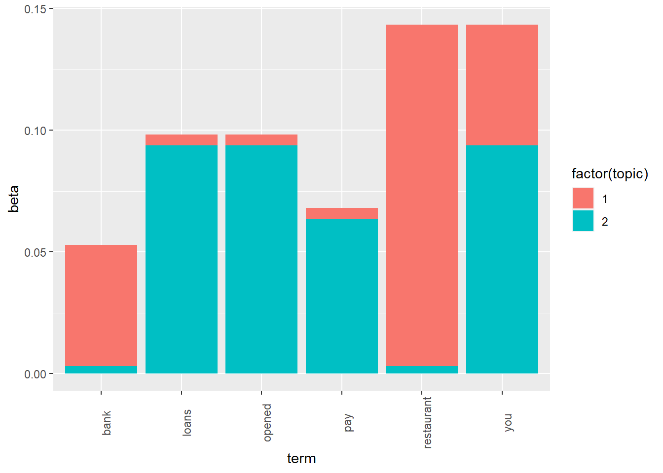
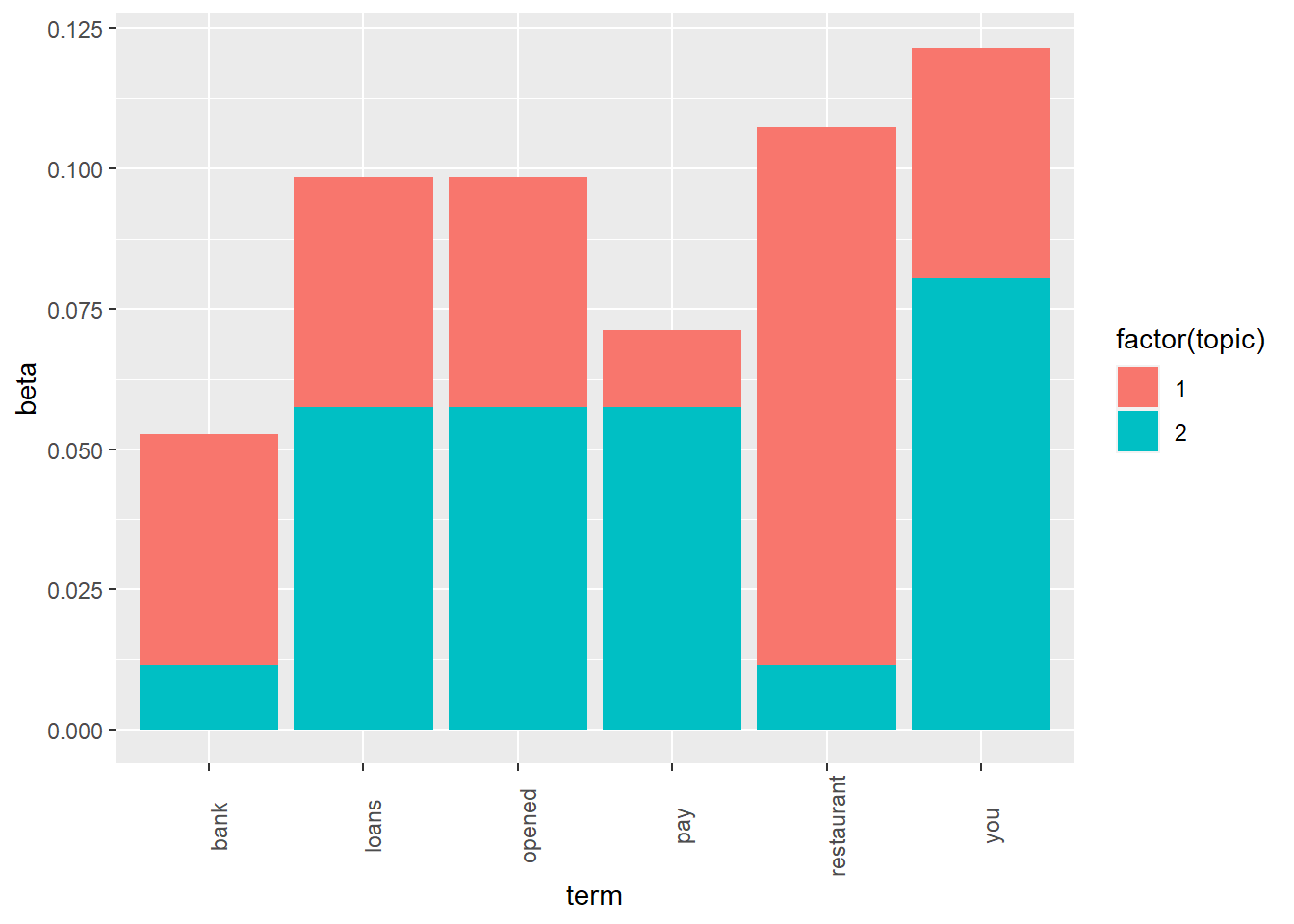
Parameter alpha determines the values of probabilities that a document belongs to a topic. Parameter delta does the same for the probability distribution of words over topics. By default, delta is set to 0.1. (Oleinikov 2019)
alpha和delta 都有这样的作用,调整整个主题模型概率分布的形状。
Corners correspond to (1,0,0), (0,1,0), and (0,0,1) combinations

image

image
Left: alpha > 1, right: alpha < 1
delta
参考 Oleinikov (2019)
Parameter alpha determines the values of probabilities that a document belongs to a topic.
alpha 是用来决定 gamma 的。
Parameter delta does the same for probability distribution of words over topics.
delta 是用来决定 bata 的。
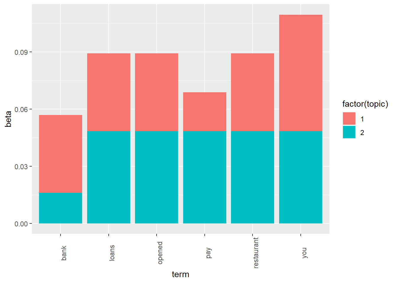
The probabilities of words are more even in the second chart, when delta was set to 0.5.
dtm <- read_rds("output/dtm.rds")

test_delta <- function(delta = 0.1){

    # Fit the model for delta = 0.5
    mod <- LDA(x=dtm, k=2, method="Gibbs",
               control=list(iter=500, seed=12345, alpha=1, delta=delta))

    # Define which words we want to examine
    my_terms = c("loans", "bank", "opened", "pay", "restaurant", "you")

    # Make a tidy table
    t <- tidy(mod, "beta") %>% filter(term %in% my_terms)

    # Make a stacked column chart
    ggplot(t, aes(x=term, y=beta)) + geom_col(aes(fill=factor(topic))) +
      theme(axis.text.x=element_text(angle=90))
}
16.3 Beta 词汇-主题概率
参考 Silge and Robinson (2019)
It treats each document as a mixture of topics, and each topic as a mixture of words.
这是最直观的理解,用“文档 \(\times\) 关键词”作为矩阵进行计算。
- Every document is a mixture of topics. We imagine that each document may contain words from several topics in particular proportions. For example, in a two-topic model we could say “Document 1 is 90% topic A and 10% topic B, while Document 2 is 30% topic A and 70% topic B.”
- Every topic is a mixture of words. For example, we could imagine a two-topic model of American news, with one topic for “politics” and one for “entertainment.” The most common words in the politics topic might be “President”, “Congress”, and “government”, while the entertainment topic may be made up of words such as “movies”, “television”, and “actor”. Importantly, words can be shared between topics; a word like “budget” might appear in both equally.
以上的矩阵中列(文档)和行(词汇)中产生主题。
## <<DocumentTermMatrix (documents: 2246, terms: 10473)>>
## Non-/sparse entries: 302031/23220327
## Sparsity           : 99%
## Maximal term length: 18
## Weighting          : term frequency (tf)
ap_lda <- LDA(AssociatedPress, k = 2, control = list(seed = 1234))
ap_lda
ap_lda %>% write_rds("output/ap_lda.rds")感觉模型的构建有点慢。
we introduced the
tidy()method, originally from the broom package (Robinson 2017), for tidying model objects. The tidytext package provides this method for extracting the per-topic-per-word probabilities, called
\(\beta\) (“beta”), from the model.
既然是个概率,一定是正数,越大越好。
Notice that this has turned the model into a one-topic-per-term-per-row format. For each combination, the model computes the probability of that term being generated from that topic. For example, the term “aaron” has a \(1.686917 \times 10^{−12}\) probability of being generated from topic 1, but a \(3.8959408 \times 10^{−5}\) probability of being generated from topic 2.
这样解释就清楚多了。
ap_top_terms <- ap_topics %>%
  group_by(topic) %>%
  top_n(10, beta) %>%
  ungroup() %>%
  arrange(topic, -beta)

ap_top_terms %>%
  mutate(term = reorder(term, beta)) %>%
  ggplot(aes(term, beta, fill = factor(topic))) +
  geom_col(show.legend = FALSE) +
  facet_wrap(~ topic, scales = "free") +
  coord_flip()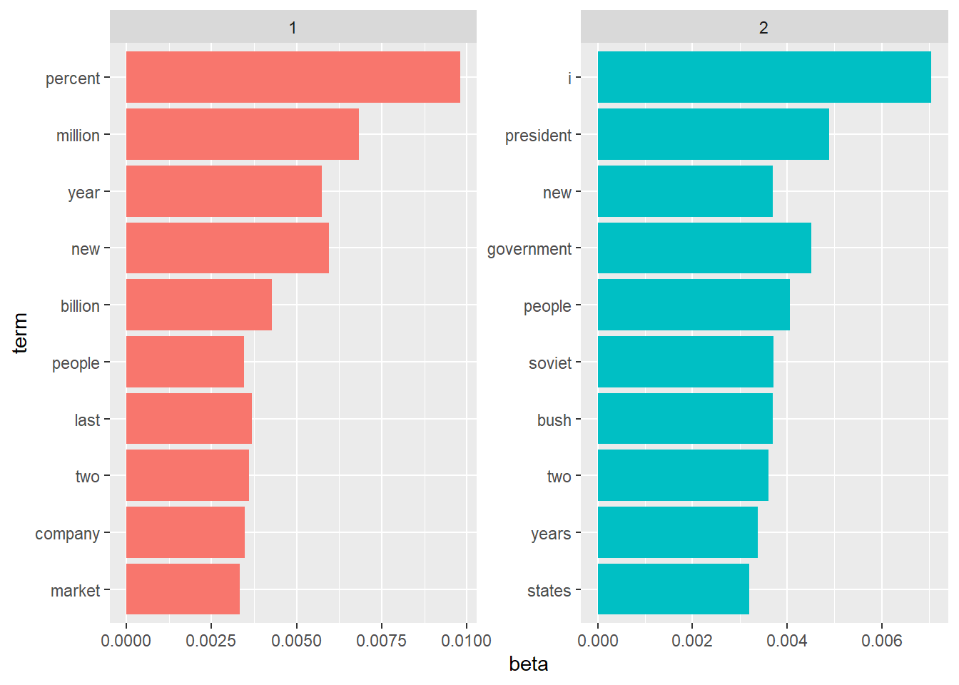
scales = "free"即可。
One important observation about the words in each topic is that some words, such as “new” and “people”, are common within both topics. This is an advantage of topic modeling as opposed to “hard clustering” methods: topics used in natural language could have some overlap in terms of words.
这是主题模型作为聚类的优秀之处,考虑了主题重叠的情况。
beta_spread <- ap_topics %>%
  mutate(topic = paste0("topic", topic)) %>%
  spread(topic, beta) %>%
  dplyr::filter(topic1 > .001 | topic2 > .001) %>%
  mutate(log_ratio = log2(topic2 / topic1))

beta_spread %>%
    arrange(desc(log_ratio))
所以 topic 2 更加偏政治,topic 1 更加偏金融。
16.4 Gamma 文档-主题概率
… per-document-per-topic probabilities, called \(\gamma\) (“gamma”)
Each of these values is an estimated proportion of words from that document that are generated from that topic. For example, the model estimates that only about 24.8% of the words in document 1 were generated from topic 1.
这里的 Gamma 衡量的是所有词汇-主题相加后,得到的。
17 主题模型训练
18 主题模型可视化
18.1 主题-词汇
数据清洗,参考 Silge and Robinson (2019)
lda_model %>%
    tidytext::tidy(matrix = 'beta') %>%
    group_by(topic) %>%
    top_n(20, beta) %>%
    ungroup() %>%
    arrange(topic, -beta) -> lda_beta_top
可视化的思路参考 GitHub 和 Prevos (2018)
棒棒糖图参考 r_eda lollipop
lda_beta_top %>%
    mutate(topic = as.factor(topic)) %>%
    group_by(topic) %>%
    mutate(term = fct_reorder(term, beta)) %>%
    ggplot() +
    aes(term, beta, fill = topic) +
    geom_point(show.legend = FALSE) +
    geom_segment(aes(x = term, xend = term,
                     y = 0, yend = beta)) +
    scale_fill_manual(values = wesanderson::wes_palette("Royal1")) +
    facet_wrap(~topic, scales = "free") +
    coord_flip() +
    theme_minimal() +
    theme(text = element_text(size = 8))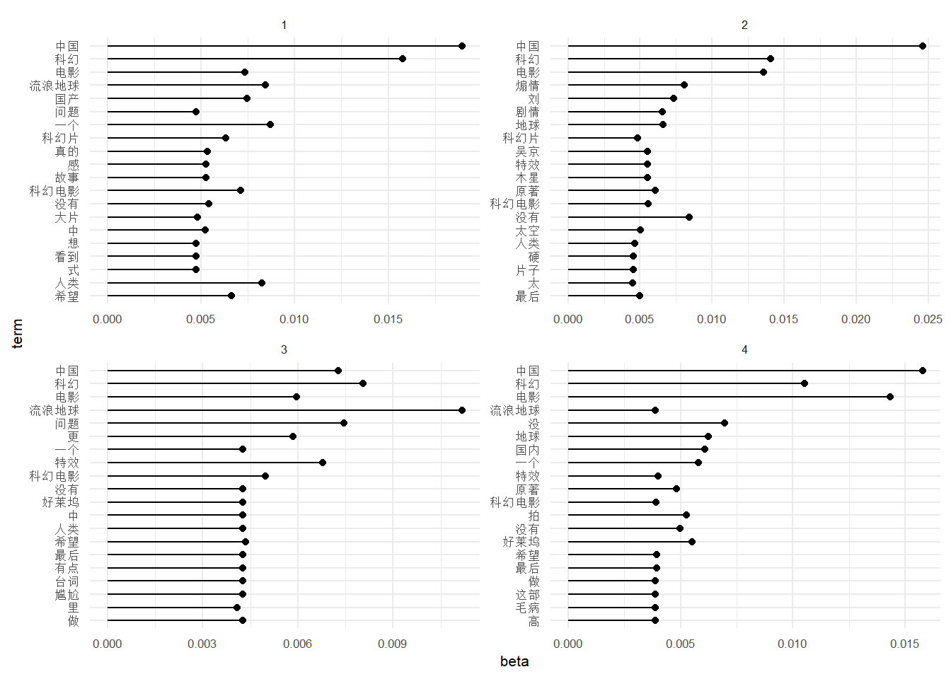
18.1.1 矩阵展示
参考 Oleinikov (2019)
##      Topic 1      Topic 2
## [1,] "opened"     "you"
## [2,] "restaurant" "loans"
## [3,] "a"          "to"
## [4,] "new"        "the"
## [5,] "bank"       "off"
这反馈一个 matrix,非常的内存节省。
## $`Topic 1`
## [1] "a"          "new"        "opened"     "restaurant"
##
## $`Topic 2`
## [1] "loans" "to"    "off"   "pay"   "the"   "you"   "will"
18.2 主题-文档
参考 Oleinikov (2019)
# Extract matrix gamma and plot it
tidy(mod, "gamma") %>%
    mutate(document=as.numeric(document)) %>%
    ggplot(aes(x=document, y=gamma)) +
    geom_line(aes(color=factor(topic))) +
    labs(x="Chapter", y="Topic probability") +
    scale_color_manual(values=brewer.pal(n=4, "Set1"), name="Topic")
# include_graphics("refs/topics-line-plot.png")
include_graphics("https://jiaxiangbu.github.io/learn_nlp/datacamp/topic-modeling-in-r/refs/topics-line-plot.png")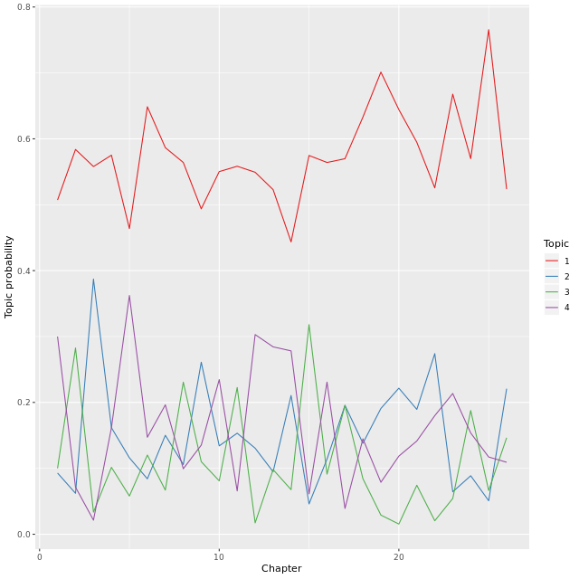
这比 bar 图更加清晰,但是可以看到每个章节都是 topic 1 占领。
19 LDA 主题数确定
参考 Pleplé (2013),Perplexity 的评价方式是一个 held-out 的思想,将文本数据集分为 train 和 test,针对 train 组训练得到 \(\alpha\) (文档的主题分布的超参数)、\(\mathbf{\Phi}\) (主题矩阵)。 然后针对 test 进行预测,评价指标为
\[\begin{align} \mathcal{L}(\boldsymbol{w})=\log p(\boldsymbol{w} | \mathbf{\Phi}, \alpha)=\sum_{d} \log p\left(\boldsymbol{w}_{d} | \mathbf{\Phi}, \alpha\right) \tag{19.1} \end{align}\]
公式 (19.1) 是一个条件概率公式,\(\mathcal{L}(\boldsymbol{w})\) 衡量文档 \(\boldsymbol{w}\) 的 log 可能性,因此越大越好。
\[\begin{align} \text{ perplexity } ( \text{test set } \boldsymbol{w} )=\exp \left\{-\frac{\mathcal{L}(\boldsymbol{w})}{\text { count of tokens }}\right\} \tag{19.2} \end{align}\]
公式 (19.2) 这是一个负相关函数,因此 perplexity 越小越好。
20 sklearn 框架
情感分析调用预训练模型、主题模型展示。
21 gensim 框架
22 NLP英文小例子
参考 Oleinikov (2019)
dtm <- corpus %>%
    # Specify the input column
    unnest_tokens(input=text, output=word, drop=TRUE) %>%
    dplyr::count(id, word) %>%
    # Specify the token
cast_dtm(document=id, term=word, value=n)对于英文文档,unnest_tokens起到了分词的作用,但是对于中文,计算 dtm 也就是这样一个词频矩阵,还是需要 jiebaR 先分词才行。
## [1] "DocumentTermMatrix" "simple_triplet_matrix"## <<DocumentTermMatrix (documents: 5, terms: 31)>>
## Non-/sparse entries: 44/111
## Sparsity : 72%
## Maximal term length: 10
## Weighting : term frequency (tf)## Terms
## Docs bad due loans to are bank if late off pay the you your a downtown in new
## 1 1 1 1 1 0 0 0 0 0 0 0 0 0 0 0 0 0
## 2 0 0 1 2 1 1 1 1 1 1 1 1 1 0 0 0 0
## 3 0 0 0 0 0 0 0 0 0 0 0 0 0 1 1 1 1
## 4 0 0 0 0 0 0 0 0 0 0 0 0 0 1 0 0 1
## 5 0 0 1 0 0 0 0 0 1 1 2 3 0 0 0 0 0
## Terms
## Docs opened restaurant is just on street that there warwick for how need want
## 1 0 0 0 0 0 0 0 0 0 0 0 0 0
## 2 0 0 0 0 0 0 0 0 0 0 0 0 0
## 3 1 1 0 0 0 0 0 0 0 0 0 0 0
## 4 1 1 1 1 1 1 1 1 1 0 0 0 0
## 5 1 1 0 0 0 0 0 0 0 1 1 1 1
## Terms
## Docs will
## 1 0
## 2 0
## 3 0
## 4 0
## 5 2这个矩阵记录的是词频。
cast_dtm 函数把df转换成 dtm。
mod = LDA(x=dtm, k=2, method="Gibbs", control=list(alpha=1, delta=0.1, seed=10005))

posterior(mod)$topics
## 1 2
## 1 0.1666667 0.8333333
## 2 0.1428571 0.8571429
## 3 0.8750000 0.1250000
## 4 0.8461538 0.1538462
## 5 0.2222222 0.777777822.1 doc with topics matrix to np.array
23 动态主题模型
区别于静态的LDA,动态LDA更能够反应随着时间变化,主题的更新、新增、消失(Blei and Lafferty 2006)。
使用模块 from gensim.models.wrappers.dtmmodel import DtmModel 可以完成,但是这只是一个封装函数,需要外部下载预测脚本。
数据输入只比静态LDA多了一个时间维度。
并且可以作为一个预测模型,预测下一个时间窗口的主题。
主题的可视化参考 Cai-Pincus (2017) 和 Svitlana (2019)
Building prefix dict from the default dictionary ...
Loading model from cache C:\Users\LIJIAX~1\AppData\Local\Temp\jieba.cache
Loading model cost 0.954 seconds.
Prefix dict has been built succesfully.| Group | Students | Content | text | |
|---|---|---|---|---|
| 0 | 第1组 | 正三 | 慕课将分布于世界各地的最优质的教育资源聚集到一起,让任何有学习愿望的人能够低成本的,通常是免… | 慕课 将 分布 于 世界各地 的 最 优质 的 教育资源 聚集 到 一起 , 让 任何 有 … |
| 1 | 第1组 | 正二 | 在慕课发展过程中的现阶段,中国最大的慕课平台icourse163的用户人数突破100万,与其… | 在 慕课 发展 过程 中 的 现阶段 , 中国 最大 的 慕课 平台 icourse163 … |
| 2 | 第1组 | 正一 | 研究发现,在慕课融入的课堂学习中,学习者情感体验丰富,知识技能以及元认知能力得到提升,思想观… | 研究 发现 , 在 慕课 融入 的 课堂 学习 中 , 学习者 情感 体验 丰富 , 知识 … |
| 3 | 第1组 | 正三 | 慕课在保证教育质量的同时,降低提供教育的成本,给社会带来的憧憬。任何人任何时候再任何地方,都… | 慕课 在 保证 教育 质量 的 同时 , 降低 提供 教育 的 成本 , 给 社会 带来 的… |
| 4 | 第1组 | 正一 | 对方反一辩友也说是可能出现的欢快气氛,传统课堂集体聆听教师单方面赐予的知识,这难道不是一种容… | 对方 反一 辩友 也 说 是 可能 出现 的 欢快 气氛 , 传统 课堂 集体 聆听 教师 … |
series_slices = affirmative['Group'] \
    .value_counts() \
    .reindex(affirmative['Group'].unique().tolist()) \
    .tolist()
# regex https://pandas.pydata.org/pandas-docs/stable/reference/api/pandas.Series.str.replace.html
# reindex https://blog.csdn.net/songyunli1111/article/details/78953841[67, 135, 50, 53, 50, 47, 53, 68, 63, 31]
stopwords = get_custom_stopwords("stopwords.txt", encoding='utf-8') # HIT停用词词典
max_df = 0.9 # 在超过这一比例的文档中出现的关键词(过于平凡),去除掉。
min_df = 5 # 在低于这一数量的文档中出现的关键词(过于独特),去除掉。
n_features = 1000 # 最大提取特征数量
n_top_words = 20 # 显示主题下关键词的时候,显示多少个
col_content = "text" # 说明其中的文本信息所在列名称# 参考 https://blog.csdn.net/kwame211/article/details/78963517
import jieba
docs = [[word for word in jieba.cut(document, cut_all=True)] for document in raw_documents]# 参考 https://radimrehurek.com/gensim/auto_examples/tutorials/run_lda.html#sphx-glr-auto-examples-tutorials-run-lda-py
from gensim.corpora import Dictionary
# Create a dictionary representation of the documents.
dictionary = Dictionary(docs)
# Filter out words that occur less than 5 documents, or more than 90% of the documents.
dictionary.filter_extremes(no_below=5, no_above=0.9)print('Number of unique tokens: %d' % len(dictionary))
print('Number of documents: %d' % len(corpus))Number of unique tokens: 1060 Number of documents: 617
from gensim.models.wrappers import DtmModel

# Set training parameters.
num_topics = 8
chunksize = 2000
passes = 20
iterations = 400
eval_every = None  # Don't evaluate model perplexity, takes too much time.

# Make a index to word dictionary.
temp = dictionary[0]  # This is only to "load" the dictionary.
id2word = dictionary.id2token

# 参考 https://radimrehurek.com/gensim/models/wrappers/dtmmodel.html
# dtm-win64.exe

model = DtmModel('dtm-win64.exe', corpus=corpus, id2word=id2word, num_topics = num_topics,
                 time_slices=series_slices)
# 参考 https://github.com/le-hoang-nhan/dynamic-topic-modeling
print(model.show_topic(topicid=1, time=0, topn=10))[(0.054934152899280886, ‘学习’), (0.046114835910420926, ‘课’), (0.04495083634524851, ‘慕’), (0.0318348783258449, ‘课程’), (0.01555991198548604, ‘和’), (0.011949879053584214, ‘是’), (0.01155140324098257, ‘方式’), (0.011004917227570849, ‘在’), (0.010536307542231893, ‘学习者’), (0.009003648555199277, ‘可以’)]
#Topic Evolution
num_topics = 8
for topic_no in range(num_topics):
    print("\nTopic", str(topic_no))
    for time in range(len(series_slices)):
        print("Time slice", str(time))
        print(model.show_topic(topic_no, time, topn=10))
Topic 0 Time slice 0 [(0.04018052022066546, ‘课’), (0.036249815551255456, ‘慕’), (0.02448548586657437, ‘是’), (0.023714387154559223, ‘发展’), (0.02367722760054125, ‘教育’), (0.017694317247958412, ‘我们’), (0.015624579186324783, ‘传统’), (0.015025505230014904, ‘在’), (0.012114008172785072, ‘了’), (0.011049820951041131, ‘反’)] Time slice 1 [(0.039142497272909985, ‘课’), (0.03579706784786207, ‘慕’), (0.024401378796314526, ‘是’), (0.023846475526857383, ‘教育’), (0.022735096814248044, ‘发展’), (0.017555946228496894, ‘我们’), (0.01571500622082442, ‘传统’), (0.014949393473384368, ‘在’), (0.012299193140748553, ‘了’), (0.010744284499093485, ‘反’)] Time slice 2 [(0.038475424316991955, ‘课’), (0.035365687723283065, ‘慕’), (0.024247191229078716, ‘是’), (0.023408284563598707, ‘教育’), (0.021401225289811407, ‘发展’), (0.01754042821642195, ‘我们’), (0.015669111450072614, ‘传统’), (0.014988245923534156, ‘在’), (0.01251012095645997, ‘了’), (0.010650328460717643, ‘反’)] Time slice 3 [(0.03748845503205829, ‘课’), (0.03517131753550811, ‘慕’), (0.024461251639387362, ‘是’), (0.024118862139508646, ‘教育’), (0.020929886702576266, ‘发展’), (0.01706426482217534, ‘我们’), (0.01573990448113794, ‘传统’), (0.014856137599769914, ‘在’), (0.012719443112197188, ‘了’), (0.010138173852388431, ‘反’)] Time slice 4 [(0.03719956491215089, ‘课’), (0.035290416211194414, ‘慕’), (0.025577216048735932, ‘是’), (0.0240259509842123, ‘教育’), (0.02086623092779554, ‘发展’), (0.016692516659497936, ‘我们’), (0.015499920030568425, ‘传统’), (0.014401604929428916, ‘在’), (0.012803289667194061, ‘了’), (0.010367010546146112, ‘反’)] Time slice 5 [(0.0376826194695201, ‘课’), (0.035774161892084565, ‘慕’), (0.02675996855888743, ‘是’), (0.023724244461838465, ‘教育’), (0.02080540762639873, ‘发展’), (0.016608311268597385, ‘我们’), (0.015114441677050285, ‘传统’), (0.014014529379079564, ‘在’), (0.012305422088176176, ‘了’), (0.010279117179744756, ‘不是’)] Time slice 6 [(0.0380057490915557, ‘课’), (0.036296136528269476, ‘慕’), (0.026791016720672512, ‘是’), (0.023744384403670403, ‘教育’), (0.02110898533796707, ‘发展’), (0.01656172928143064, ‘我们’), (0.014965581519263162, ‘传统’), (0.013993372054708401, ‘在’), (0.012119372474888, ‘了’), (0.010682494297792671, ‘辩’)] Time slice 7 [(0.038809426760298915, ‘课’), (0.036867924714266684, ‘慕’), (0.026766904852246236, ‘是’), (0.024315922723598976, ‘教育’), (0.021868373469311135, ‘发展’), (0.017137449222767172, ‘我们’), (0.015033427474279827, ‘传统’), (0.01420528404581441, ‘在’), (0.011840247918862798, ‘了’), (0.010990547491185498, ‘辩’)] Time slice 8 [(0.038580897427402186, ‘课’), (0.037051905575546926, ‘慕’), (0.026579425103050842, ‘是’), (0.02453537343655193, ‘教育’), (0.021962475958624956, ‘发展’), (0.01807394044474617, ‘我们’), (0.01529447563982258, ‘传统’), (0.014488114864041364, ‘在’), (0.011615441835162927, ‘了’), (0.01135836831016874, ‘辩’)] Time slice 9 [(0.03770843483239827, ‘课’), (0.03690376025702986, ‘慕’), (0.026726106859098108, ‘是’), (0.024348138459742683, ‘教育’), (0.021670702225834185, ‘发展’), (0.018777215787530464, ‘我们’), (0.015553666336518921, ‘传统’), (0.014558912535715729, ‘在’), (0.011971136330618892, ‘辩’), (0.011524312780100625, ‘了’)]
Topic 1 Time slice 0 [(0.054934152899280886, ‘学习’), (0.046114835910420926, ‘课’), (0.04495083634524851, ‘慕’), (0.0318348783258449, ‘课程’), (0.01555991198548604, ‘和’), (0.011949879053584214, ‘是’), (0.01155140324098257, ‘方式’), (0.011004917227570849, ‘在’), (0.010536307542231893, ‘学习者’), (0.009003648555199277, ‘可以’)] Time slice 1 [(0.05378748380817899, ‘学习’), (0.0463546716000786, ‘课’), (0.045166205835513444, ‘慕’), (0.031113446909549963, ‘课程’), (0.015231093816602745, ‘和’), (0.011786945612377794, ‘是’), (0.01122449310144545, ‘方式’), (0.011190497543014585, ‘在’), (0.010385574216791132, ‘学习者’), (0.009063335720296092, ‘可以’)] Time slice 2 [(0.052337378630711244, ‘学习’), (0.04629567360034417, ‘课’), (0.04523467343564046, ‘慕’), (0.030580889840616136, ‘课程’), (0.01501764824452899, ‘和’), (0.011644947540786849, ‘是’), (0.011355641733286063, ‘在’), (0.010895479730929681, ‘方式’), (0.010250350009989369, ‘学习者’), (0.00911814978325485, ‘可以’)] Time slice 3 [(0.052019197033386706, ‘学习’), (0.045178180919502216, ‘课’), (0.044093763829961476, ‘慕’), (0.030174693479521567, ‘课程’), (0.014708104473342495, ‘和’), (0.011600651274844902, ‘在’), (0.011566732748848552, ‘是’), (0.010734122077021822, ‘方式’), (0.01001148460211611, ‘学习者’), (0.00921047775032469, ‘可以’)] Time slice 4 [(0.05197608370038308, ‘学习’), (0.04470391950991499, ‘课’), (0.043750749567985865, ‘慕’), (0.029795846855142787, ‘课程’), (0.01420839423212455, ‘和’), (0.011856074355156915, ‘在’), (0.0115989077539342, ‘是’), (0.010192721424754653, ‘方式’), (0.009785142853016094, ‘学习者’), (0.009368429450202638, ‘可以’)] Time slice 5 [(0.05211423874967438, ‘学习’), (0.04412865107617742, ‘课’), (0.04326048874903337, ‘慕’), (0.02945986423276053, ‘课程’), (0.01378440350693095, ‘和’), (0.012031901312498728, ‘在’), (0.0116682473042017, ‘是’), (0.009664176257045666, ‘方式’), (0.009603386090185257, ‘学习者’), (0.009491420237252883, ‘可以’)] Time slice 6 [(0.05264320361635566, ‘学习’), (0.04312590267960136, ‘课’), (0.042197909821724215, ‘慕’), (0.029270162183748682, ‘课程’), (0.013321776542459893, ‘和’), (0.012235716178717685, ‘在’), (0.011647073759958536, ‘是’), (0.009611384126215096, ‘可以’), (0.009468385922424383, ‘学习者’), (0.00919775051182748, ‘方式’)] Time slice 7 [(0.05334984517457836, ‘学习’), (0.04290268045892763, ‘课’), (0.04193635971813644, ‘慕’), (0.029034378904558344, ‘课程’), (0.013050310269502919, ‘和’), (0.012302496705468962, ‘在’), (0.0115159246074654, ‘是’), (0.009741190102050015, ‘可以’), (0.009239317193142355, ‘学习者’), (0.00890501075545838, ‘方式’)] Time slice 8 [(0.0539659591010802, ‘学习’), (0.04225209487474747, ‘课’), (0.04114642727610467, ‘慕’), (0.027941870000560164, ‘课程’), (0.012880496975186867, ‘和’), (0.012442429554416512, ‘在’), (0.011453170940297576, ‘是’), (0.009757764670364268, ‘可以’), (0.009206115229903755, ‘学习者’), (0.008717169030553959, ‘方式’)] Time slice 9 [(0.0541402205078836, ‘学习’), (0.042266719998823025, ‘课’), (0.04099104452745667, ‘慕’), (0.028029889607110014, ‘课程’), (0.012890672907732706, ‘和’), (0.012420446961624533, ‘在’), (0.011441577079463331, ‘是’), (0.009730321180510844, ‘可以’), (0.009265681958486056, ‘学习者’), (0.008726559951221364, ‘方式’)]
Topic 2 Time slice 0 [(0.031043233122451754, ‘学生’), (0.02668271222856447, ‘老师’), (0.023868882330323894, ‘课堂’), (0.01978205010813496, ‘讲’), (0.01947673094819849, ‘了’), (0.019325452802306416, ‘在’), (0.01836283686644334, ‘传统’), (0.017318549706166055, ‘再’), (0.015891868788748716, ‘教师’), (0.015160064584276909, ‘让’)] Time slice 1 [(0.031161923143938907, ‘学生’), (0.02679014682954436, ‘老师’), (0.024430861703648603, ‘课堂’), (0.019668971079179608, ‘讲’), (0.01953602185460035, ‘了’), (0.01953219556291146, ‘在’), (0.01868839445476059, ‘传统’), (0.017088586720705526, ‘再’), (0.015892732200471212, ‘教师’), (0.01494692860725533, ‘让’)] Time slice 2 [(0.03118943500842519, ‘学生’), (0.027117189963761935, ‘老师’), (0.023904497846617863, ‘课堂’), (0.01978769569436053, ‘了’), (0.0196096782419648, ‘讲’), (0.019434566586155787, ‘在’), (0.018299114325817135, ‘传统’), (0.017339243225109966, ‘再’), (0.015902369485761448, ‘教师’), (0.015318567610544455, ‘让’)] Time slice 3 [(0.03146207517707275, ‘学生’), (0.02742492624227265, ‘老师’), (0.023483130241425978, ‘课堂’), (0.019893874039512153, ‘了’), (0.019676272597791204, ‘讲’), (0.01934814542767233, ‘在’), (0.017959498585997786, ‘传统’), (0.01756348666457092, ‘再’), (0.015942490689198726, ‘教师’), (0.015703911593576033, ‘让’)] Time slice 4 [(0.0317100864289313, ‘学生’), (0.027738456787464626, ‘老师’), (0.023066658337744787, ‘课堂’), (0.020002668335331125, ‘了’), (0.019745094989990605, ‘讲’), (0.019266201455595253, ‘在’), (0.017779973055643758, ‘再’), (0.017605206280777913, ‘传统’), (0.016077397443412075, ‘让’), (0.015994447397268723, ‘教师’)] Time slice 5 [(0.03193941357759384, ‘学生’), (0.028447449176350347, ‘老师’), (0.02265880188688491, ‘课堂’), (0.02002530202843254, ‘讲’), (0.019956568354989657, ‘了’), (0.019240421642298236, ‘在’), (0.01808640653395788, ‘再’), (0.01723517903792803, ‘传统’), (0.01632024388626679, ‘让’), (0.015973972926436205, ‘教师’)] Time slice 6 [(0.032099608456050234, ‘学生’), (0.029155990026305617, ‘老师’), (0.022461505512630733, ‘课堂’), (0.020237600956090125, ‘讲’), (0.019878779030697902, ‘了’), (0.019306864978632293, ‘在’), (0.01822756137849164, ‘再’), (0.01703195388674161, ‘传统’), (0.016462770874924607, ‘让’), (0.016020733284440453, ‘教师’)] Time slice 7 [(0.03200701229302776, ‘学生’), (0.02959003560566229, ‘老师’), (0.02221169409800385, ‘课堂’), (0.020485273210613098, ‘讲’), (0.01975131748116563, ‘了’), (0.019375568293687966, ‘在’), (0.018461646990408854, ‘再’), (0.0168586118632216, ‘传统’), (0.016684886515355397, ‘让’), (0.016036007942597557, ‘教师’)] Time slice 8 [(0.03196072928049309, ‘学生’), (0.02972941942350236, ‘老师’), (0.022021051722567197, ‘课堂’), (0.0208463718282348, ‘讲’), (0.019661829773081573, ‘了’), (0.019384936799303008, ‘在’), (0.018735002126184005, ‘再’), (0.01698352944469504, ‘让’), (0.01667377209645531, ‘传统’), (0.01590745085674958, ‘教师’)] Time slice 9 [(0.031948524181557296, ‘学生’), (0.029781288544860632, ‘老师’), (0.022015662600748376, ‘课堂’), (0.02092500817038431, ‘讲’), (0.0196502208979976, ‘了’), (0.019389988248985097, ‘在’), (0.018718304836340568, ‘再’), (0.016970055481089222, ‘让’), (0.01667398274960847, ‘传统’), (0.015896487252398755, ‘教师’)]
Topic 3 Time slice 0 [(0.03478450059729968, ‘学生’), (0.03308917916908039, ‘互动’), (0.030603703132624425, ‘课’), (0.025994683760542776, ‘视频’), (0.025381439726455745, ‘慕’), (0.02498397518628086, ‘在’), (0.02484427503006549, ‘过程’), (0.019060681696505235, ‘中’), (0.018504091742821055, ‘交流’), (0.016644809503940445, ‘可以’)] Time slice 1 [(0.03491737023070852, ‘学生’), (0.033089149150791766, ‘互动’), (0.030807850914277003, ‘课’), (0.02607037410149659, ‘视频’), (0.025687451828533405, ‘慕’), (0.024782668335654647, ‘在’), (0.02443723378926502, ‘过程’), (0.019148774506294444, ‘交流’), (0.01912800693667351, ‘中’), (0.01656879784893786, ‘可以’)] Time slice 2 [(0.03482743395249812, ‘学生’), (0.03375835158900804, ‘互动’), (0.03122387504674024, ‘课’), (0.026017449047841586, ‘慕’), (0.025524407507364007, ‘视频’), (0.02466529610396268, ‘在’), (0.023888748979799018, ‘过程’), (0.01908688331026287, ‘交流’), (0.01868888970711729, ‘中’), (0.01658193522001172, ‘可以’)] Time slice 3 [(0.034609321682797935, ‘学生’), (0.0342883978435074, ‘互动’), (0.03163370962214529, ‘课’), (0.026332736453291143, ‘慕’), (0.024892817388217192, ‘视频’), (0.024562578049403, ‘在’), (0.023445760329839804, ‘过程’), (0.0189128151006007, ‘交流’), (0.018208491529166145, ‘中’), (0.016541577519618024, ‘可以’)] Time slice 4 [(0.0353252242952848, ‘互动’), (0.0342997316407563, ‘学生’), (0.03194609447687641, ‘课’), (0.026708311420545347, ‘慕’), (0.02421236532800773, ‘在’), (0.024142967461078194, ‘视频’), (0.022978080381951208, ‘过程’), (0.01892704494027778, ‘交流’), (0.017842107088248696, ‘中’), (0.01648291085757951, ‘可以’)] Time slice 5 [(0.03668934984535697, ‘互动’), (0.034189088673073305, ‘学生’), (0.0320994745335359, ‘课’), (0.02702006012222778, ‘慕’), (0.023841090156256645, ‘在’), (0.02361417113989999, ‘视频’), (0.02251838383540359, ‘过程’), (0.01901099847822973, ‘交流’), (0.01745843845695539, ‘中’), (0.01649212600639042, ‘可以’)] Time slice 6 [(0.03754054929791722, ‘互动’), (0.03403096791294207, ‘学生’), (0.032020443564574314, ‘课’), (0.027077051252370348, ‘慕’), (0.02378554729819673, ‘在’), (0.023100156347330324, ‘视频’), (0.022173398235200887, ‘过程’), (0.019230544738786118, ‘交流’), (0.017353524425428826, ‘大学’), (0.01722480406671932, ‘中’)] Time slice 7 [(0.037250013804589775, ‘互动’), (0.03383928473922231, ‘学生’), (0.03203839596942005, ‘课’), (0.027150803851453627, ‘慕’), (0.023693067946479934, ‘在’), (0.022439759731971067, ‘视频’), (0.02209728003132034, ‘过程’), (0.019328806931718942, ‘交流’), (0.01859817060185241, ‘大学’), (0.01712489376857812, ‘中’)] Time slice 8 [(0.03752095503814028, ‘互动’), (0.03376632424974765, ‘学生’), (0.0318823991326904, ‘课’), (0.02702942619527794, ‘慕’), (0.023453615727353574, ‘在’), (0.022040791909604857, ‘过程’), (0.021968402693487776, ‘视频’), (0.019450549943356293, ‘交流’), (0.018517436544249095, ‘大学’), (0.017077551189938766, ‘可以’)] Time slice 9 [(0.03718718236008152, ‘互动’), (0.033602296871603925, ‘学生’), (0.03195427350782894, ‘课’), (0.027039622922568538, ‘慕’), (0.02339159644133195, ‘在’), (0.022011466482721516, ‘过程’), (0.021857962562173337, ‘视频’), (0.019370521257706653, ‘交流’), (0.018561464671929432, ‘大学’), (0.017027237803033952, ‘中’)]
Topic 4 Time slice 0 [(0.04956667978235987, ‘课堂’), (0.04224031253737317, ‘传统’), (0.030989743667082993, ‘课’), (0.029442439609799375, ‘慕’), (0.020647403012586173, ‘有’), (0.018652282664530315, ‘是’), (0.01816217128905854, ‘学生’), (0.01558067270671716, ‘可以’), (0.013339358449420673, ‘就’), (0.011650113714919252, ‘会’)] Time slice 1 [(0.04851821170332693, ‘课堂’), (0.0412023720316644, ‘传统’), (0.031068041945627466, ‘课’), (0.029455084723486503, ‘慕’), (0.020570173565022845, ‘有’), (0.018792678410578172, ‘是’), (0.018080195057368745, ‘学生’), (0.015782070728338985, ‘可以’), (0.013308550409014684, ‘就’), (0.011642484162246147, ‘会’)] Time slice 2 [(0.04739151497583057, ‘课堂’), (0.03949821981303601, ‘传统’), (0.030649425056184385, ‘课’), (0.02882567441251896, ‘慕’), (0.020131305276954403, ‘有’), (0.019148481326168306, ‘是’), (0.018326226194356667, ‘学生’), (0.0157172137302653, ‘可以’), (0.013278139501223064, ‘就’), (0.011545830569594694, ‘会’)] Time slice 3 [(0.04667880234751612, ‘课堂’), (0.03853463205330011, ‘传统’), (0.030045044082842354, ‘课’), (0.028383934610094516, ‘慕’), (0.019727496692280046, ‘有’), (0.01928725498708801, ‘是’), (0.018712722645918365, ‘学生’), (0.015599564170647371, ‘可以’), (0.012838483134456917, ‘就’), (0.011491684171162727, ‘会’)] Time slice 4 [(0.04804990945565695, ‘课堂’), (0.03853064891137565, ‘传统’), (0.0298416952152532, ‘课’), (0.028259088079953955, ‘慕’), (0.01954310212081199, ‘是’), (0.019093320466999377, ‘有’), (0.018926002170655164, ‘学生’), (0.01538500334857041, ‘可以’), (0.012398825915660414, ‘就’), (0.011707212256965761, ‘教学’)] Time slice 5 [(0.04920305511247075, ‘课堂’), (0.03854866946866856, ‘传统’), (0.030251675682522926, ‘课’), (0.028607554372619092, ‘慕’), (0.0200750165995673, ‘是’), (0.018748092888301263, ‘学生’), (0.018297287091093694, ‘有’), (0.01500285349051558, ‘可以’), (0.012144628948766369, ‘教学’), (0.01201398160527892, ‘就’)] Time slice 6 [(0.04973450304804439, ‘课堂’), (0.03825840577501354, ‘传统’), (0.030102370389858683, ‘课’), (0.028290328763368962, ‘慕’), (0.020326847137202807, ‘是’), (0.01874187535427461, ‘学生’), (0.017761945724526464, ‘有’), (0.014790098822473716, ‘可以’), (0.012273386608105343, ‘教学’), (0.011985297239336692, ‘就’)] Time slice 7 [(0.05003350805417175, ‘课堂’), (0.0384093473946478, ‘传统’), (0.030361171400892024, ‘课’), (0.028280602704762604, ‘慕’), (0.02049494050881725, ‘是’), (0.01874143588771648, ‘学生’), (0.017422130453253096, ‘有’), (0.014541705623562337, ‘可以’), (0.012464317554868865, ‘教学’), (0.012092387979076327, ‘就’)] Time slice 8 [(0.04960942467340186, ‘课堂’), (0.03836084247757951, ‘传统’), (0.03065095414412935, ‘课’), (0.028263142113815212, ‘慕’), (0.02061842238029155, ‘是’), (0.018687752667659614, ‘学生’), (0.017200061062186137, ‘有’), (0.014404855687894463, ‘可以’), (0.012793043432952362, ‘教学’), (0.012246965430597575, ‘就’)] Time slice 9 [(0.04781898043692375, ‘课堂’), (0.03781216995864401, ‘传统’), (0.03107454153882952, ‘课’), (0.028405899626330756, ‘慕’), (0.020682323913433158, ‘是’), (0.01866982715292522, ‘学生’), (0.017239815756473178, ‘有’), (0.014414672082684304, ‘可以’), (0.012958271047437565, ‘教学’), (0.012337656412479692, ‘就’)]
Topic 5 Time slice 0 [(0.06060419612650297, ‘学生’), (0.043216792104618804, ‘教学’), (0.035737970897222054, ‘教师’), (0.03567803892402352, ‘学习’), (0.014708231902937062, ‘课堂’), (0.01411506576462234, ‘是’), (0.014028544623039207, ‘在’), (0.01265644236102711, ‘能力’), (0.012295212902863803, ‘和’), (0.012156331913353767, ‘知识’)] Time slice 1 [(0.06105087877647187, ‘学生’), (0.044565810950528306, ‘教学’), (0.035444678531413434, ‘学习’), (0.0347215291771198, ‘教师’), (0.014779978085309942, ‘课堂’), (0.013990843484638327, ‘在’), (0.013918606005572322, ‘是’), (0.012602800340250547, ‘能力’), (0.012405199212411766, ‘和’), (0.012139345223738768, ‘知识’)] Time slice 2 [(0.06377632175694446, ‘学生’), (0.04652650826707044, ‘教学’), (0.03468844929301224, ‘学习’), (0.0341440988246698, ‘教师’), (0.014752438214906155, ‘课堂’), (0.013983753905181352, ‘在’), (0.013929639444474553, ‘是’), (0.012728576483715054, ‘能力’), (0.012263422901288826, ‘和’), (0.011893910752090942, ‘模式’)] Time slice 3 [(0.06673793538594877, ‘学生’), (0.048514483739755976, ‘教学’), (0.034150504095303964, ‘学习’), (0.03372425261345089, ‘教师’), (0.014752448880067106, ‘课堂’), (0.013971482847810891, ‘在’), (0.013864115521255375, ‘是’), (0.012764374207736141, ‘能力’), (0.012133766664613334, ‘和’), (0.011994153573461694, ‘模式’)] Time slice 4 [(0.06934554255201682, ‘学生’), (0.04864865497346316, ‘教学’), (0.03347404146831549, ‘学习’), (0.03314665981609522, ‘教师’), (0.0146487602855706, ‘课堂’), (0.013935162772140762, ‘在’), (0.013726206660217776, ‘是’), (0.013027375511886222, ‘能力’), (0.012097404138502662, ‘和’), (0.01188071695366726, ‘模式’)] Time slice 5 [(0.07176439230106732, ‘学生’), (0.04861568001103926, ‘教学’), (0.03298934300692353, ‘学习’), (0.03264986437349297, ‘教师’), (0.014437768493920628, ‘课堂’), (0.013915249370771546, ‘在’), (0.013548626508142972, ‘是’), (0.013378601062486966, ‘能力’), (0.011978144331790095, ‘和’), (0.011639549658911638, ‘模式’)] Time slice 6 [(0.0740077841281674, ‘学生’), (0.04760514166500249, ‘教学’), (0.03259553871921955, ‘学习’), (0.03257998902106331, ‘教师’), (0.01427382917788545, ‘课堂’), (0.013946609113212974, ‘在’), (0.013708529665585, ‘能力’), (0.013327273506684901, ‘是’), (0.011846117819348781, ‘和’), (0.011460607173706307, ‘模式’)] Time slice 7 [(0.07462689846685222, ‘学生’), (0.04745812947910056, ‘教学’), (0.03270772889455349, ‘教师’), (0.03217099166392202, ‘学习’), (0.014161228686801995, ‘能力’), (0.014114761884021014, ‘课堂’), (0.014030964376361947, ‘在’), (0.01310384230486897, ‘是’), (0.01177615193247913, ‘和’), (0.011477426026532142, ‘模式’)] Time slice 8 [(0.07423183310934998, ‘学生’), (0.04784872713045115, ‘教学’), (0.031642903074736606, ‘学习’), (0.030973189489815364, ‘教师’), (0.014693065329761364, ‘能力’), (0.014132142186785907, ‘在’), (0.01394899824409272, ‘课堂’), (0.012993708491849184, ‘是’), (0.011792234342879493, ‘和’), (0.011576685544675043, ‘自主’)] Time slice 9 [(0.0730782453231518, ‘学生’), (0.04925066607150434, ‘教学’), (0.03175177721767025, ‘学习’), (0.030609128836988377, ‘教师’), (0.014673648679346953, ‘能力’), (0.014195170313593377, ‘在’), (0.013943549611241545, ‘课堂’), (0.012959333553791334, ‘是’), (0.011767854097003084, ‘模式’), (0.011735592906837964, ‘和’)]
Topic 6 Time slice 0 [(0.05163670101389453, ‘学习’), (0.039370766625564775, ‘学生’), (0.03259497150886033, ‘是’), (0.02150376877644676, ‘可以’), (0.019106275565166583, ‘自己’), (0.018344581173411933, ‘欠’), (0.016783309461376503, ‘反驳’), (0.01494834696286401, ‘视频’), (0.013994675551937017, ‘课’), (0.013363667304837543, ‘反方’)] Time slice 1 [(0.05245498712399898, ‘学习’), (0.03969828217102865, ‘学生’), (0.031937251908131126, ‘是’), (0.021567188911449413, ‘可以’), (0.018958992103236438, ‘自己’), (0.018397103739622177, ‘欠’), (0.017058928191157587, ‘反驳’), (0.014946688167272897, ‘视频’), (0.01398375917210308, ‘课’), (0.013733396763071181, ‘反方’)] Time slice 2 [(0.048992630981370085, ‘学习’), (0.04112400674103026, ‘学生’), (0.03115211276534384, ‘是’), (0.021936398644385322, ‘可以’), (0.019218255370484764, ‘自己’), (0.016549932573453576, ‘欠’), (0.015910782575657412, ‘反驳’), (0.014524080253095173, ‘视频’), (0.014216209164617287, ‘课’), (0.01282352997170056, ‘老师’)] Time slice 3 [(0.047338252395502746, ‘学习’), (0.0425851191638865, ‘学生’), (0.030510602024756004, ‘是’), (0.021803699352687177, ‘可以’), (0.019476639756585857, ‘自己’), (0.01470352437886155, ‘反驳’), (0.014700061674155373, ‘欠’), (0.014213914996909232, ‘课’), (0.01413716973973845, ‘视频’), (0.013132364996910655, ‘老师’)] Time slice 4 [(0.044980232915000015, ‘学习’), (0.044278936707761625, ‘学生’), (0.030355010693182596, ‘是’), (0.021276408503533198, ‘可以’), (0.01949881712659191, ‘自己’), (0.014226233500737302, ‘课’), (0.013749577330715905, ‘反驳’), (0.013618928405139187, ‘视频’), (0.013567430139041355, ‘老师’), (0.013267884392706803, ‘欠’)] Time slice 5 [(0.046542466783302726, ‘学生’), (0.043341923708613776, ‘学习’), (0.030628530420590713, ‘是’), (0.02063519894177178, ‘可以’), (0.01924756362459158, ‘自己’), (0.01425522367709233, ‘课’), (0.013961789776545445, ‘老师’), (0.01342515299201269, ‘视频’), (0.013026419154332178, ‘课堂’), (0.01280662383943072, ‘反驳’)] Time slice 6 [(0.0488105600202176, ‘学生’), (0.042984296600448314, ‘学习’), (0.03038761464384281, ‘是’), (0.020511145527460722, ‘可以’), (0.01924292113289597, ‘自己’), (0.014438066586704382, ‘老师’), (0.014281191579100566, ‘课’), (0.013177119889773421, ‘视频’), (0.012975925479537522, ‘课堂’), (0.012125276752964926, ‘反驳’)] Time slice 7 [(0.05045658875083782, ‘学生’), (0.04217913070932786, ‘学习’), (0.030036857861200396, ‘是’), (0.02052572727261513, ‘可以’), (0.019222984420198593, ‘自己’), (0.014924843221757828, ‘老师’), (0.014392841895593747, ‘课’), (0.012980427881244965, ‘课堂’), (0.012934105160393195, ‘视频’), (0.012197489310306524, ‘慕’)] Time slice 8 [(0.051307536356148084, ‘学生’), (0.04156904229273555, ‘学习’), (0.029732613380863124, ‘是’), (0.020177545789701587, ‘可以’), (0.018914589650024724, ‘自己’), (0.0151516991137321, ‘老师’), (0.01448618337428118, ‘课’), (0.013068968240775636, ‘课堂’), (0.012873355926496523, ‘视频’), (0.01231552723110718, ‘慕’)] Time slice 9 [(0.0512201671629085, ‘学生’), (0.04179591897765148, ‘学习’), (0.029294289592098604, ‘是’), (0.020006315979417075, ‘可以’), (0.018640658775284227, ‘自己’), (0.015077638094101918, ‘老师’), (0.014590782553808556, ‘课’), (0.013092995150296166, ‘课堂’), (0.012764127777530838, ‘视频’), (0.01241143705382842, ‘慕’)]
Topic 7 Time slice 0 [(0.04155050025586591, ‘课’), (0.0412813609322021, ‘教育’), (0.04113811434564692, ‘慕’), (0.029891036515182472, ‘学生’), (0.02238701299242733, ‘了’), (0.021779309260608472, ‘可以’), (0.015046215294124383, ‘高等教育’), (0.015028681375320511, ‘高等’), (0.014030820011552739, ‘学习’), (0.013864929224113294, ‘有’)] Time slice 1 [(0.041798526340811624, ‘课’), (0.04128450773035317, ‘慕’), (0.04107703998028797, ‘教育’), (0.030073561771584278, ‘学生’), (0.02200268648175038, ‘了’), (0.021899768205864978, ‘可以’), (0.015252865079998993, ‘高等教育’), (0.01523586318192207, ‘高等’), (0.014107872237227861, ‘有’), (0.01396806112024677, ‘学习’)] Time slice 2 [(0.042502504918615534, ‘课’), (0.0420973127564189, ‘慕’), (0.04143910339591302, ‘教育’), (0.030839843636242762, ‘学生’), (0.022074763546659937, ‘了’), (0.020892907186399898, ‘可以’), (0.014537339118450078, ‘高等教育’), (0.014524818797632358, ‘高等’), (0.014277249337845174, ‘资源’), (0.01421622093527994, ‘学习’)] Time slice 3 [(0.04336037488889295, ‘课’), (0.043019223155686945, ‘慕’), (0.04217081355234577, ‘教育’), (0.031834898341413016, ‘学生’), (0.02223215208296449, ‘了’), (0.01970321994935713, ‘可以’), (0.014938683395219449, ‘资源’), (0.014556664147741157, ‘学习’), (0.013919650454365141, ‘高等教育’), (0.013911846076770885, ‘高等’)] Time slice 4 [(0.044985600467996274, ‘课’), (0.044633909083057165, ‘慕’), (0.04294086905530461, ‘教育’), (0.030981940509531413, ‘学生’), (0.021396228806589625, ‘了’), (0.0193921168332304, ‘可以’), (0.015452699037040434, ‘资源’), (0.014535477212555875, ‘学习’), (0.013888082810001793, ‘有’), (0.013734997994375196, ‘高等教育’)] Time slice 5 [(0.04658509756624165, ‘课’), (0.046223764050351945, ‘慕’), (0.04411095953656606, ‘教育’), (0.030128033731712495, ‘学生’), (0.02047817323118304, ‘了’), (0.019091738065197865, ‘可以’), (0.015946139320227405, ‘资源’), (0.014468456572948542, ‘学习’), (0.01397983072872993, ‘有’), (0.013605724133333826, ‘高等教育’)] Time slice 6 [(0.047641410926043196, ‘课’), (0.04721963516081467, ‘慕’), (0.04491122550932498, ‘教育’), (0.029638634069458738, ‘学生’), (0.019507496046990654, ‘了’), (0.01905952129173672, ‘可以’), (0.016516524065443128, ‘资源’), (0.01442484722694525, ‘学习’), (0.014022551618687207, ‘有’), (0.013328919360854945, ‘高等教育’)] Time slice 7 [(0.048752589060081564, ‘课’), (0.04844521171508396, ‘慕’), (0.045518772093486, ‘教育’), (0.028992330192367605, ‘学生’), (0.019075426359530828, ‘可以’), (0.018787586672248637, ‘了’), (0.017023198398977285, ‘资源’), (0.014394605586039314, ‘学习’), (0.013999393568927302, ‘有’), (0.01308198735709312, ‘高等教育’)] Time slice 8 [(0.04936880492973243, ‘课’), (0.04901112859508301, ‘慕’), (0.045682778203039044, ‘教育’), (0.028536398422748972, ‘学生’), (0.019043136945138178, ‘可以’), (0.01886500550255054, ‘了’), (0.017119903497492112, ‘资源’), (0.014247205688250735, ‘学习’), (0.014012229409575796, ‘有’), (0.013044438517886864, ‘高等教育’)] Time slice 9 [(0.04942533673998944, ‘课’), (0.04903613764260683, ‘慕’), (0.04574936592230411, ‘教育’), (0.028485591641290522, ‘学生’), (0.01905844807149583, ‘可以’), (0.01892528829440913, ‘了’), (0.017392264071679275, ‘资源’), (0.01421055053582155, ‘学习’), (0.013985860381756856, ‘有’), (0.013011959774260038, ‘高等教育’)]
#Distance between documents: compare the documents across different time-frames and see how similar they are topic-wise
#considering document 0
doc = 0
print("doc = 0, model.gamma_[doc]",model.gamma_[doc])
doc = 0, model.gamma_[doc] [1.88394876e-04 7.01846241e-01 1.88394876e-04 1.88394876e-04 1.88595226e-01 1.88394876e-04 1.88394876e-04 1.08616559e-01]
#The distance between documents based on their topic distribution: lower, more related

from gensim.matutils import hellinger
# considering document 4 and 5
doc1 = 4
doc2 = 5
hellinger(model.gamma_[doc1], model.gamma_[doc2])
0.8113757952202133
import pyLDAvis

doc_topic, topic_term, doc_lengths, term_frequency, vocab = model.dtm_vis(time=0, corpus=corpus)
vis_wrapper = pyLDAvis.prepare(topic_term_dists=topic_term, doc_topic_dists=doc_topic, doc_lengths=doc_lengths, vocab=vocab, term_frequency=term_frequency)
pyLDAvis.display(vis_wrapper)
D:-packages_prepare.py:257: FutureWarning: Sorting because non-concatenation axis is not aligned. A future version of pandas will change to not sort by default.
To accept the future behavior, pass ‘sort=False’.
To retain the current behavior and silence the warning, pass ‘sort=True’.
return pd.concat([default_term_info] + list(topic_dfs))
<class ‘gensim.models.wrappers.dtmmodel.DtmModel’>
24 Debug DTM
24.2 method=‘fixed’
如果 corpus 出现[] 空 list 的情况,会报错。
raise ValueError("""There is a text without words in the input corpus.
This breaks method='fixed' (The DIM model).""")
目前分析的问题是
- 可能 text 字太少,字典解析的时候为空
- 字都太常见,因此字典内不含有这种高频不常见的词
24.3 其他
要学会查看源代码。
D:\install\miniconda\Lib\site-packages\~ensim\models\wrappers\dtmmodel.py
corpus ({iterable of list of (int, float), scipy.sparse.csc}) – Stream of document vectors or sparse matrix of shape (num_terms, num_documents). https://radimrehurek.com/gensim/models/ldaseqmodel.html
找到原因了, 因为一个样本字数不够,也会报错。
returned non-zero exit status 1.
还有一个 slice 文档太少也不行。 否则 num_topic 太多 fit 不出来。
总结来说,就是样本量和样本内字数在每个 slice 里面要充足。
24.4 model = ‘dtm’
常常 By T By Topic 的对象为空。
25 主题相似性
参考 python - How to plot a heatmap from pandas DataFrame - Stack Overflow 我觉得不好,不使用。
参考 python 3.x - Topic Similarity in one model to csv Matrix - Stack Overflow
kullback_leibler不对称,其他都对称,都是距离,越小越相似。
kullback_leibler
          1         2         3         4         5
1  0.000000  0.886015  0.880052  0.836047  0.885342
2  0.866027  0.000000  0.846337  0.827272  0.892016
3  0.871223  0.815762  0.000000  0.812200  0.836045
4  0.846152  0.884209  0.868788  0.000000  0.913046
5  0.781929  0.909090  0.884018  0.863445  0.000000
hellinger
          1         2         3         4         5
1  0.000000  0.990853  0.997136  0.994644  0.961479
2  0.990853  0.000000  0.959581  0.991588  0.977318
3  0.997136  0.959581  0.000000  0.995260  0.966042
4  0.994644  0.991588  0.995260  0.000000  0.997639
5  0.961479  0.977318  0.966042  0.997639  0.000000
jaccard
          1         2         3         4         5
1  0.000000  0.817530  0.825107  0.839990  0.817530
2  0.817530  0.000000  0.709960  0.770068  0.736386
3  0.825107  0.709960  0.000000  0.809861  0.761808
4  0.839990  0.770068  0.809861  0.000000  0.727692
5  0.817530  0.736386  0.761808  0.727692  0.000000
jensen_shannon
          1         2         3         4         5
1  0.000000  0.983271  0.995298  0.991134  0.931214
2  0.983271  0.000000  0.923467  0.985689  0.955231
3  0.995298  0.923467  0.000000  0.993487  0.937346
4  0.991134  0.985689  0.993487  0.000000  0.997544
5  0.931214  0.955231  0.937346  0.997544  0.000000
后面三个都是对称的。
参考 https://radimrehurek.com/gensim/auto_examples/tutorials/run_distance_metrics.html 计算主题距离。
topic_over_topic, annotation = lda.diff(lda, annotation=True)
df_topic_over_topic = pd.DataFrame(topic_over_topic)KL散度,越小越好,说明越相似。
参考 python - How to plot a heatmap from pandas DataFrame - Stack Overflow
import matplotlib.pyplot as plt
import seaborn as sns
ax = sns.heatmap(df_topic_over_topic)

plt.yticks(np.arange(0.5, len(df_topic_over_topic.index), 1), df_topic_over_topic.index)
plt.xticks(np.arange(0.5, len(df_topic_over_topic.columns), 1), df_topic_over_topic.columns)

# turn the axis label
for item in ax.get_yticklabels():
    item.set_rotation(0)

for item in ax.get_xticklabels():
    item.set_rotation(90)

# save figure
plt.savefig('output/heatmap_topic_over_topic.png', dpi=100)
plt.show()
png
这个也可以去计算话题演化 26。
25.1 PCA
这里展示的图都是用 PCA 度量距离的,实际过程中发现了和 KL 的差异还蛮大的。
d:-packages_testing.py:19: FutureWarning: pandas.util.testing is deprecated. Use the functions in the public API at pandas.testing instead. import pandas.util.testing as tm
The blackcellmagic extension is already loaded. To reload it, use: %reload_ext blackcellmagic
indices = np.arange(len(corpus))
np.random.shuffle(indices)
# sub_corpus = [i for i in corpus if len(i)>10]
some_corpus = corpus[indices.tolist()][:10000]
doc_term_matrix = get_doc_term_matrix(some_corpus,dictionary)
corpus_output = lda.get_document_topics(doc_term_matrix)(gensim.interfaces.TransformedCorpus, 10000)
Note: if you’re in the IPython notebook, pyLDAvis.show() is not the best command to use. Consider using pyLDAvis.display(), or pyLDAvis.enable_notebook(). See more information at http://pyLDAvis.github.io/quickstart.html .
You must interrupt the kernel to end this command
Serving to http://127.0.0.1:8889/ [Ctrl-C to exit]
127.0.0.1 - - [10/Jul/2020 18:37:02] “GET / HTTP/1.1” 200 - 127.0.0.1 - - [10/Jul/2020 18:37:02] “GET /LDAvis.css HTTP/1.1” 200 - 127.0.0.1 - - [10/Jul/2020 18:37:02] “GET /d3.js HTTP/1.1” 200 - 127.0.0.1 - - [10/Jul/2020 18:37:03] “GET /LDAvis.js HTTP/1.1” 200 - 127.0.0.1 - - [10/Jul/2020 18:37:04] code 404, message Not Found 127.0.0.1 - - [10/Jul/2020 18:37:04] “GET /favicon.ico HTTP/1.1” 404 -
stopping Server…
[NbConvertApp] Converting notebook lda-short-text-topic-distance.ipynb to html [NbConvertApp] Writing 430631 bytes to output-short-text-topic-distance.html
26 话题演化
构建一种微博话题演化方法, 正确把握话题发展趋势, 提高网络舆情预警能力。【 方法】使用 Skip-gram 模型在文本集上训练得到词向量模型, 将每一时间片的微博文本输入 BTM 得到候选主题, 在主题维 上构造候选主题词向量; 利用K-means算法对主题词向量聚类, 得到融合后的主题, 进而建立文本集在时间片上 的话题演化路径。
其实类似于动态主题模型,其中在文献综述部分也提及,
另一方面, 研究人员将时间信息引入LDA模型, 研究话题随时间的动态迁移, 如 Topic over Time (ToT)模型、动态话题模型。齐亚双等利用DTM 模型分析学科领域研究方向和发展演化情况;
张佩瑶 and 刘东苏 (2019) 并且采用以上端到端的做法,而是,
使用 Skip-gram 模型训练整个语料库, 得到相应 词汇的词向量; 将 BTM 得到的每一时间片的候选主 题词表示为主题词向量, 主题词向量利用语料库中丰 富的语义信息评估词语的相似性。
skip-gram 训练词向量。 BTM/LDA 训练主题模型,每个主题选择 Top K 的关键词。一般地,主题之间含有相同的关键词,但是排序不一样。 因此要区分主题之间的差异,应该考虑这种排序的顺序。
这个时候引入训练好的词向量,去表达每个主题里面关键词的词向量。 这里的做法是把主题们看成等长度的序列特征。
将词表 \(T_{i}\) 中的词汇输入到词向量模型中,获得词表 \(T_{i}\) 中每一个词的词向量表 \(T_{-} w 2 v=\left\{w_{m}, v\left(w_{m}\right), w_{m} \in T_{i}\right\}\) 将 \(T_{-} w 2 v\) 输入 K-means 进行聚类;
这里可以不使用 K—Means。先说 张佩瑶 and 刘东苏 (2019) 的目的。
假设我们有10个主题,每个主题选择 Top 20 的词汇,那么样本集合是 (10,20)。 我们有词向量,假设有10000个词,每个词可以表达为300维度,因此词向量大小为(10000,300)。 我们从中选出我们需要的10个主题Top 20 的词汇,最后样本变成 (10,20,300)。 显然我们为了简化,需要样本变为(10,300),这一步降维的操作,就是一个主题表达为(,300)维度。 然后我们可以利用这300维度,去计算每个主题之间的相关性。
这里可以用
- KMeans
- Doc2Vec
以新浪微博“勒索病毒”话题为例, 选取主题之 间相似度阈值为 0.5, 确定相邻时间片主题之间的 演化关系, 从主题内容方面进行演化分析, 包括 主题的新生、合并、孤立和消亡等情况, 结果如图 4 所示。
演化是通过相关性来确定的。
最后计算主题相似度, 完成话题演化分析。
这一步才是关键,相关性卡了相关性,比如绝对值小于0.5,就算不相连。
整体的思路如图
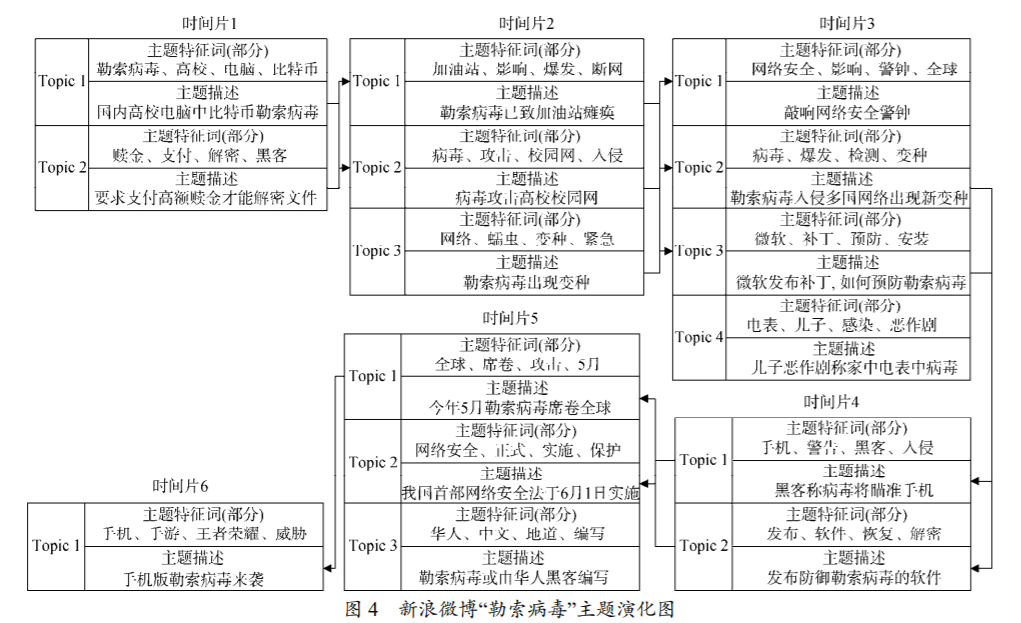
Figure 26.1: 新浪微博“勒索病毒”主题演化图
以下复现这个过程。
import pandas as pd
import numpy as np

# 保存模型
import pickle as pkl

# 调用词向量
from gensim.models import KeyedVectors

# 降维
from sklearn.cluster import KMeans

# 文学编程
# %load_ext blackcellmagictime_range_list = []
time_range_name_list = []
for idx,lda in enumerate(lda_list):
doc2vec_list = []
chn_name_list = []
for i in range(lda.num_topics):
words = [lda.id2word[i[0]] for i in lda.get_topic_terms(i, topn=30)]
embed_value_list = []
for word in words:
try:
embed_value = zh_model.get_vector(word)
# embed_value = embed_value.reshape(1,-1)
except:
embed_value = np.random.uniform(0,1,300)
# 如果不存在就随机给
embed_value_list.append(embed_value)
doc2vec = KMeans(n_clusters=1).fit(np.row_stack(embed_value_list)).cluster_centers_
print('lda id'+str(idx+1))
print('topic id'+str(i+1))
print(doc2vec.shape)
chn_name01 = '-'.join(words[0:5])
chn_name02 = '-'.join(words[6:10])
chn_name = '\n'.join([chn_name01,chn_name02])
doc2vec_list.append(doc2vec)
chn_name_list.append(chn_name)
# = pd.Dataframe(doc2vec_list, columns = range(lda.num_topics))
time_range_list.append(doc2vec_list)
time_range_name_list.append(chn_name_list)lda id1 topic id1 (1, 300) lda id1 topic id2 (1, 300) lda id1 topic id3 (1, 300) lda id1 topic id4 (1, 300) lda id1 topic id5 (1, 300) lda id2 topic id1 (1, 300) lda id2 topic id2 (1, 300) lda id2 topic id3 (1, 300) lda id2 topic id4 (1, 300) lda id2 topic id5 (1, 300) lda id3 topic id1 (1, 300) lda id3 topic id2 (1, 300) lda id3 topic id3 (1, 300) lda id3 topic id4 (1, 300) lda id3 topic id5 (1, 300) lda id4 topic id1 (1, 300) lda id4 topic id2 (1, 300) lda id4 topic id3 (1, 300) lda id4 topic id4 (1, 300) lda id4 topic id5 (1, 300) lda id5 topic id1 (1, 300) lda id5 topic id2 (1, 300) lda id5 topic id3 (1, 300) lda id5 topic id4 (1, 300) lda id5 topic id5 (1, 300) lda id6 topic id1 (1, 300) lda id6 topic id2 (1, 300) lda id6 topic id3 (1, 300) lda id6 topic id4 (1, 300) lda id6 topic id5 (1, 300) lda id7 topic id1 (1, 300) lda id7 topic id2 (1, 300) lda id7 topic id3 (1, 300) lda id7 topic id4 (1, 300) lda id7 topic id5 (1, 300) lda id8 topic id1 (1, 300) lda id8 topic id2 (1, 300) lda id8 topic id3 (1, 300) lda id8 topic id4 (1, 300) lda id8 topic id5 (1, 300)
(8, 5)
a = np.array(
    [
        [["aA1", "aA2", "aA3"], ["aB1", "aB2", "aB3"]],
        [["bA1", "bA2", "bA3"], ["bB1", "bB2", "bB3"]],
        [["cA1", "cA2", "cA3"], ["cB1", "cB2", "cB3"]],
    ]
)
a
array([[[‘aA1’, ‘aA2’, ‘aA3’], [‘aB1’, ‘aB2’, ‘aB3’]],
 [['bA1', 'bA2', 'bA3'],
        ['bB1', 'bB2', 'bB3']],

       [['cA1', 'cA2', 'cA3'],
['cB1', 'cB2', 'cB3']]], dtype='<U3')array([[‘aA1’, ‘aA2’, ‘aA3’], [‘aB1’, ‘aB2’, ‘aB3’], [‘bA1’, ‘bA2’, ‘bA3’], [‘bB1’, ‘bB2’, ‘bB3’], [‘cA1’, ‘cA2’, ‘cA3’], [‘cB1’, ‘cB2’, ‘cB3’]], dtype=‘<U3’)
output_array = np.array(time_range_list).reshape(8,5,300).reshape(8*5,300).transpose()
name_array = np.array(time_range_name_list).reshape(8*5).tolist()(300, 40)
column_name = ['Time'+str(i)+'_Topic'+str(j) for i in range(8) for j in range(5)]
column_name = [i+'\n'+j for i,j in zip(column_name,name_array)]生成好主题之间的序列特征嵌入后,进行相关性度量。 这里主题的关键词进行了脱敏。
corr_df <-
    df %>%
    cor() %>%
    data.frame(check.names = F, check.rows = F) %>%
    rownames_to_column(var = "left") %>%
write_excel_csv("../data/lda-w2v-corr.csv")pca_df <-
pca_model$x %>%
as.data.frame() %>%
rownames_to_column('name') %>%
dplyr::select(1:3) %>%
mutate(id = str_extract(name, pattern = "Time\\d_Topic\\d")) %>%
mutate(time_first = str_detect(name, "Time[0246]"))
pca_df %>%
ggplot(aes(
x = PC1,
y = PC2,
col = time_first,
label = name
)) +
geom_point() +
geom_text() +
# stat_ellipse() +
theme_classic() +
labs(title = '各主题 相似度')
time_first区分时间切片是第一,还是第二进入。
Time4和Time6是一类人的说的话吧,可以认为和另外一类人差异大。
但是关键词不只是五个啊,考虑了30个,只是展示不方便,只给了5个。
pca_df %>%
    mutate(t_id = str_extract(name,"Time\\d") %>% str_extract("\\d")) %>%
    ggplot(aes(
        x = t_id,
        y = PC1,
        col = time_first,
        label = name
    )) +
    geom_point() +
    geom_text() +
    stat_ellipse() +
    theme_classic() +
    labs(title = '各主题 BY BIN 相似度')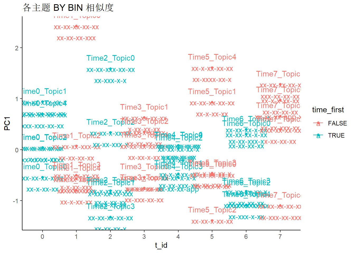
corr_df_sub <-
    corr_df %>%
    gather(right, value,-left) %>%
    mutate(left_t_id = str_extract(left,"Time\\d") %>% str_extract("\\d") %>% as.integer(),
           right_t_id = str_extract(right,"Time\\d") %>% str_extract("\\d") %>% as.integer()) %>%
    filter(left_t_id==right_t_id-1) %>%
    filter(value < 1, value > .8)
dim(corr_df_sub)
## [1] 49 5link_text <-
corr_df_sub %>%
mutate(text = glue::glue("'{left}' -> '{right}'")) %>%
mutate(text = str_replace_all(text,"\\n","\\\\n")) %>%
summarise(text = str_flatten(text, "\n")) %>%
dplyr::pull()
# cat(link_text)entry_text <-
corr_df_sub %>%
select(1:2) %>%
gather() %>%
dplyr::pull(value) %>%
unique()
entry_text <-
data.frame(entry_text) %>%
mutate(entry_text = glue::glue("'{entry_text}'")) %>%
mutate(entry_text = str_replace_all(entry_text,"\\n","\\\\n")) %>%
mutate(bin = str_extract(entry_text, "Time\\d")) %>%
group_by(bin) %>%
dplyr::summarise(entry_text = str_flatten(entry_text, "\n")) %>%
mutate(bin_id = str_extract(bin,"\\d")) %>%
mutate(
text = glue::glue(
"subgraph cluster<<bin_id>>{
label = '<<bin>>'
style = dashed
rank = same
}",
.open = "<<",
.close = ">>"
)
) %>%
summarise(str_flatten(text, "\n")) %>%
dplyr::pull()viz_text <- glue::glue("digraph course {
rankdir = LR
node [shape = box, style=filled]
layout = dot
compound =true
#color = crimson
}",
.open = "<<",
.close = ">>")## digraph course {
## rankdir = LR
## node [shape = box, style=filled]
## layout = dot
## compound =true
## #color = crimson
##
##
##
##
## }27 CTM
Blei, Ng, & Jordan (2003) proposed latent Dirichlet allocation (LDA) as a means of modeling documents with multiple topics but assumes the topic are uncorrelated. Blei & Lafferty (2007) proposed correlated topics model (CTM), extending LDA to allow for correlations between topics. Roberts, Stewart, Tingley, & Airoldi (2013) propose a Structural Topic Model (STM), allowing the inclusion of meta-data in the modeling process.
所以整体来说,还是要做 CTM 更好,不能假设 LDA。
from https://github.com/bab2min/tomotopy/blob/master/examples/ctm_network.py
'''
This example shows how to perform a Correlated Topic Model using tomotopy
and visualize the correlation between topics.


Required Packages:
    nltk, sklearn, pyvis
'''
import tomotopy as tp
import nltk
from nltk.corpus import stopwords
import re
from sklearn.datasets import fetch_20newsgroups
import pyvis
from pyvis.network import Network[[‘tomotopy’, ‘0.8.1’], [‘pyvis’, ‘0.1.8.1.1’]]
df = pd.read_csv('../../demo-chinese-text-classification-lstm-keras/dianping.csv')
df['text'] = df.comment.apply(lambda x: " ".join(jieba.cut(x)))
Building prefix dict from the default dictionary … Loading model from cache C:~1.cache Loading model cost 1.869 seconds. Prefix dict has been built succesfully.
# 停用词
stopwords = open("../../China-Japan/refs/stopwords.txt", "r", encoding="UTF-8").read().split("\n") + open(
    "../../China-Japan/refs/stopwords_XuYekai.txt", "r", encoding="UTF-8"
).read().split("\n")
stopwords.append('|')
stopwords = frozenset(stopwords)
len(stopwords)
875
2000
# https://github.com/bab2min/tomotopy/blob/af3a69fc6d44701ccf8a2712da7632bb84832d8b/example.py#L52
mdl = tp.CTModel(tw=tp.TermWeight.IDF, min_df=5, rm_top=40, k=30, corpus=corpus)
mdl.train(0)
# Since we have more than ten thousand of documents,
# setting the `num_beta_sample` smaller value will not cause an inaccurate result.
mdl.num_beta_sample = 5
print('Num docs:{}, Num Vocabs:{}, Total Words:{}'.format(
len(mdl.docs), len(mdl.used_vocabs), mdl.num_words
))
print('Removed Top words: ', *mdl.removed_top_words)Num docs:2000, Num Vocabs:1609, Total Words:30406 Removed Top words: 吃 味道 不错 菜 好吃 点 服务员 环境 菜品 服务 排队 感觉 口味 喜欢 真的 太 挺 推荐 比较 有点 觉得 ~ 号 店 上菜 小时 非常 里面 肉 家 东西 朋友 点评 这家 汤 排骨 完 最后 差 娜娜
# Let's train the model
# 迭代 100 次。
for i in range(0, 10, 2):
    print('Iteration: {:04}, LL per word: {:.4}'.format(i, mdl.ll_per_word))
    mdl.train(20)
print('Iteration: {:04}, LL per word: {:.4}'.format(1000, mdl.ll_per_word))
Iteration: 0000, LL per word: -32.93 Iteration: 0002, LL per word: -19.73 Iteration: 0004, LL per word: -19.48 Iteration: 0006, LL per word: -19.4 Iteration: 0008, LL per word: -19.37 Iteration: 1000, LL per word: -19.31
# Let's visualize the result
g = Network(width=800, height=800, font_color="#333")
correl = mdl.get_correlations().reshape([-1])
correl.sort()
top_tenth = mdl.k * (mdl.k - 1) // 10
top_tenth = correl[-mdl.k - top_tenth]
for k in range(mdl.k):
label = "#{}".format(k)
title= ' '.join(word for word, _ in mdl.get_topic_words(k, top_n=6))
print('Topic', label, title)
g.add_node(k, label=label, title=title, shape='ellipse')
for l, correlation in zip(range(k - 1), mdl.get_correlations(k)):
if correlation < top_tenth: continue
g.add_edge(k, l, value=float(correlation), title='{:.02}'.format(correlation))Topic #0 个人 好评 大众 开业 好喝 鸡蛋 Topic #1 特色 芝士 自助 提前 一般般 进 Topic #2 算 必点 再也 直接 微信 不让 Topic #3 点菜 中午 一点 满意 东北菜 前面 Topic #4 【 地方 以后 很大 手机 意面 Topic #5 超级 腻 门口 鸡 点餐 菜单 Topic #6 】 适合 炒 辣 基本 梨球 Topic #7 菜量 豆腐 以前 种类 吃饭 刚 Topic #8 进去 排 北京 几个 主食 少 Topic #9 真心 干酪 希望 快 量 小哥 Topic #10 喝 问 一下 找 本来 两次 Topic #11 锅包肉 蛏子 口感 招牌 量 久 Topic #12 态度 不好 服务态度 难吃 不要 钱 Topic #13 奶酪 面 罐子 座位 换 油腻 Topic #14 每次 甜 位置 恒隆 多人 确实 Topic #15 牛肉 贵 价格 爱 人多 甜品 Topic #16 梨 第一次 等位 好多 需要 茄子 Topic #17 鱼 虾 火 其实 喊 烩饭 Topic #18 实在 一份 不了 退 干净 嘈杂 Topic #19 饭 焗 海鲜 盘子 沙拉 催 Topic #20 天津 结账 高 桌子 便宜 火爆 Topic #21 烤 居然 熏 沙拉 简直 彩虹 Topic #22 之前 他家 真是 坐 过来 孩子 Topic #23 拉皮 上来 只能 人太多 发现 三个 Topic #24 烤肉 新鲜 评价 不行 自助餐 剩下 Topic #25 慢 总体 用餐 绝对 挺好吃 热情 Topic #26 - 餐厅 饮料 外面 还会 团购 Topic #27 蛋糕 妈妈 大悦 一家 城 几次 Topic #28 下次 没什么 倒 放 值得 柠檬 Topic #29 咸 失望 元 一直 再来 奶油
点击节点,查看主题关键词。
28 常见问题
28.1 LDA 产生的 index 报错
参考 https://stackoverflow.com/a/27261800/8625228 核心原因是模型训练和预测是 dictionary 不一样了,一般有两种情况
- 词汇表是需要根据 corpus 构建的。如果 corpus 不一样了,那么肯定不一样。
- 停用词处理方式不一样了,导致 corpus 不一样,同上。
output[30041]不存在,所以产生了 bug。
IndexError: index 5068 is out of bounds for axis 1 with size 5068 这个报错没有意义。
是 for i in output 没有这个数据导致的
都有这种问题,我知道了,在预测的时候也要剔除停用词。
doc_topics_output_list = []
for ((idx, df),i) in zip(df_len.groupby('text_level'),range(len(lda_list))):
    lda_model = lda_list[i]
    print(idx)
    print(df.shape)
    print(lda_model)

    corpus = df['content'].apply(lambda x: ' '.join(jieba.cut(x)).split()).apply(lambda x: [i for i in x if i not in stopwords]).values
    dictionary = corpora.Dictionary(corpus)
    # 中文会产生报错
    doc_term_matrix = [dictionary.doc2bow(rev) for rev in corpus]
    from gensim.models.ldamodel import LdaModel
    # Build LDA model
    doc_topics_output = lda_model.get_document_topics(doc_term_matrix)

    doc_topics_output_list.append(doc_topics_output)
这是 LDA 在做预测时候,注意这里每个 corpus 的元素都剔除了停用词,见).apply(lambda x: [i for i in x if i not in stopwords]),因此在预测时候也要做这一步,不然会出现,有一些词不存在的,但是还是进入了 corpus 作为一个 index 去索引,产生报错,常常出现在。
或者函数
28.2 TypeError: doc2bow expects an array of unicode tokens on input, not a single string
在执行报错。
这是因为 rev == ''时,作为dictionary.doc2bow的输入,需要为[rev]。
28.4 LDA 句子长度的影响

Figure 28.1: legend 表示字数超过n样本。主题模型预测后,选择最大概率的主题,用 cutoff 作为阈值去判断概率是否显著,Y 轴对应每个 cutoff 的平均值。曲线越向右上角,说明模型训练更好。可以发现整体来说,样本字数长度越高,模型效果越好。
28.5 根据词性的词汇过采样
# export
import numpy as np
import jieba
from jieba.posseg import cut as posseg
from pandas.core.common import flatten
def jieba_cut_with_pos_sampling(x,n,stopwords):
    output = []
    if x is np.nan:
        return ''
    if len(str(x)) > 0:
        x = str(x)
        # output = ' '.join(jieba.cut(x))

        for i,j in posseg(input_text):
            if str(i) not in stopwords and str(i) != '':
                if j in ['a','ad','an','d']:
                    i = [i for k in range(n)]

            output.append(i)
    output = list(flatten(output))
    return output
# jieba_cut_with_pos_sampling('xxx',5,stopwords)
# output2 = []
# for i,j in posseg('xxx'):
#     if str(i) not in stopwords and str(i) != '':
#         if j in ['a','ad','an','d']:
#             i = [i for k in range(5)]
#         print(i)
#         output2.append(i)

# print(output2)
这里只限定了形容词和副词 ['a','ad','an','d'],参考更多。
参考文献
- 使用 RMarkdown 的
child参数,进行文档拼接。 - 这样拼接以后的笔记方便复习。
- 相关问题提交到 Issue
29 Word2Vec
29.1 直观理解
有两个句子
onehot_names <-
lines %>%
    str_split(" ") %>%
    unlist() %>%
    unique()
# 唯一的词
onehot_names
## [1] "I"       "enjoy"   "playing" "TT"      "like"
window The maximum distance between the target word and its neighboring word. If your neighbor’s position is greater than the maximum window width to the left or the right, then, some neighbors would not be considered as being related to the target word. In theory, a smaller window should give you terms that are more related. Again, if your data is not sparse, then the window size should not matter too much, as long as it’s not overly narrow or overly broad. If you are not too sure about this, just use the default value. (Ganesan 2020)
这里其实假设了 windows 足够大,因此每个词都作为中心词,其他词都作为邻居。
##      I enjoy playing TT like
## [1,] 0     1       1  1    0
## [2,] 1     0       1  1    0
## [3,] 1     1       0  1    0
## [4,] 1     1       1  0    0
## [5,] 0     0       1  1    1
## [6,] 1     0       1  1    0
## [7,] 1     0       0  1    1
## [8,] 1 0 1 0 1## I enjoy playing TT like
## [1,] 1 0 0 0 0
## [2,] 0 1 0 0 0
## [3,] 0 0 1 0 0
## [4,] 0 0 0 1 0
## [5,] 1 0 0 0 0
## [6,] 0 0 0 0 1
## [7,] 0 0 1 0 0
## [8,] 0 0 0 1 0下面构神经网络
- input layer (8x5)
- hidden layer (8x3) (input x weight1)
- output layer (3x5) (hidden x weight2)
下面进行梯度下降 (这一步省略)
##         h1    h2    h3
## [1,]  3.38 -5.78 -0.98
## [2,]  1.78  3.19  3.63
## [3,] -5.65 -1.66 -0.24
## [4,]  3.11  5.18 -3.17
## [5,]  1.66  3.34  3.76
hidden_layer <- onehot_features %*% weight1
hidden_layer
## h1 h2 h3
## [1,] -0.76 6.71 0.22
## [2,] 0.84 -2.26 -4.39
## [3,] 8.27 2.59 -0.52
## [4,] -0.49 -4.25 2.41
## [5,] -0.88 6.86 0.35
## [6,] 0.84 -2.26 -4.39
## [7,] 8.15 2.74 -0.39
## [8,] -0.61 -4.10 2.54## h1 h2 h3 h4 h5
## [1,] -1.95 -2.01 8.71 -1.88 -0.78
## [2,] 7.64 -1.83 1.83 -2.21 -2.49
## [3,] 1.88 -2.07 1.19 4.40 -1.49output_layer <- hidden_layer %*% weight2
output_layer
## h1 h2 h3 h4 h5
## [1,] 53.1600 -11.2071 5.9215 -12.4323 -16.4429
## [2,] -27.1576 11.5347 -2.0435 -15.9006 11.5133
## [3,] 2.6835 -20.2860 76.1526 -23.5595 -12.1249
## [4,] -26.9837 3.7737 -9.1775 20.9177 7.3738
## [5,] 54.7844 -11.5095 5.3055 -11.9662 -16.9165
## [6,] -27.1576 11.5347 -2.0435 -15.9006 11.5133
## [7,] 4.3079 -20.5884 75.5366 -23.0934 -12.5985
## [8,] -25.3593 3.4713 -9.7935 21.3838 6.9002## h1 h2 h3 h4 h5
## [1,] 1 0.000 0 0 0.000
## [2,] 0 0.505 0 0 0.495
## [3,] 0 0.000 1 0 0.000
## [4,] 0 0.000 0 1 0.000
## [5,] 1 0.000 0 0 0.000
## [6,] 0 0.505 0 0 0.495
## [7,] 0 0.000 1 0 0.000
## [8,] 0 0.000 0 1 0.000以上是训练过程,下面是预测过程。
##         I enjoy playing TT like
## I       1     0       0  0    0
## enjoy   0     1       0  0    0
## playing 0     0       1  0    0
## TT      0     0       0  1    0
## like 0 0 0 0 1## h1 h2 h3
## I 3.38 -5.78 -0.98
## enjoy 1.78 3.19 3.63
## playing -5.65 -1.66 -0.24
## TT 3.11 5.18 -3.17
## like 1.66 3.34 3.76发现 like 和 enjoy 的词向量最接近,因此可以判断近义词。 可以发现,近义词的判断更多的是因为同义词发生的位置相同,周围的词相似。
并且维度从5降低到3,这实现了降维,
- 虽然这是一个监督学习,但是实质是 input => hidden 的一个内在逻辑。
- autoencoders 也可以实现。
这种降低维度的方法都算 embedding,如 t-SNE embedding。
29.2 理论
Word2vec is a neural network–based approach that comes in very handy in traditional text mining analysis. (Ayyadevara 2018) For now, let’s say we would like to convert the 5-dimensional input vector into a 3-dimensional vector. In such a scenario, our hidden layer has three neurons associated with it. (Ayyadevara 2018)
这本身是一个神经网络。
we’ll formulate the hypothesis as follows: Words that are related will have similar words surrounding them. (Ayyadevara 2018) For example, the words king and prince will have similar words surrounding them more often than not. Essentially, the context (the surrounding words) of the words would be similar.
两个相似的词的 NNs 是类似的,因此算法类似于 kNNs 了。
With this hypothesis, let’s look at each word as output and all the context words (surrounding words) as input. (Ayyadevara 2018)
有点类似于 GCN 的处理,Wang et al. (2019) 也做了 kNNs 类似于的监督学习,只是他的目标是相似两幅图的连接。 这里 NNs 进行了穷举的思路。
This way, we have converted the original input one-hot-encoded vector, where the distance between {enjoy, like} was high to the transformed word vector, where the distance between {enjoy, like} is small. (Ayyadevara 2018)
思路非常巧妙。
Word2vec is an approach that can help convert text words into numeric vectors. (Ayyadevara 2018) They have a neural network architecture that helps in coming up with vectors. (Ayyadevara 2018) The hidden layer in neural network is the key to generating the word vectors. (Ayyadevara 2018)
word2vec 使得文本稀疏矩阵变成了低维的密集矩阵,利用了神经网络的优势,其中的隐藏层是产生词向量的关键。
29.3 应用场景
29.4 Tencent AILab
参考苏剑林 腾讯AILab词向量 模型下载地址 https://ai.tencent.com/ailab/nlp/data/Tencent_AILab_ChineseEmbedding.tar.gz 大小为
> dir_info("../demo-chinese-text-classification-lstm-keras/refs") %>%
+     transmute(path = basename(path), size)
# A tibble: 2 x 2
  path                                         size
  <chr>                                 <fs::bytes>
1 Tencent_AILab_ChineseEmbedding.tar.gz       6.31G
2 Tencent_AILab_ChineseEmbedding.txt         15.59G
效果比较。
zh.vec:1600/1600 [==============================] - 7s 4ms/step - loss: 0.4032 - acc: 0.8313 - val_loss: 0.4158 - val_acc: 0.8200
w2v-Tencent_AILab:1600/1600 [==============================] - 6s 3ms/step - loss: 0.2360 - acc: 0.9156 - val_loss: 0.3585 - val_acc: 0.8600
这个结果明显比 zh.vec 好很多。
demo 如下。
29.5 增量训练
增量训练也成为 Online training / Resuming training,针对于词向量,在原来预训练的情况下,增加新的样本继续训练。
You may need to tweak the total_words parameter to train(), depending on what learning rate decay you want to simulate. Note that it’s not possible to resume training with models generated by the C tool, load_word2vec_format(). You can still use them for querying/similarity, but information vital for training (the vocab tree) is missing there. (Řehůřek 2014)
参考 Stack Overflow
调用使用load_word2vec_format的话,就不能再训练了,因为只能使用到词向量的相似性等,因为 embedding 还在,但是词汇树等都没有保存。
并且进行运算时,需要设置total_words。
预训练模型来自 Kyubyong/wordvectors (1,700Stars)
下载地址 GitHub Release 或者 Google Drive
30 Doc2Vec
Mikilov和Le使用的概念很简单,但很聪明:他们使用了word2vec模型,并添加了另一个向量(下面的段落ID),如下所示: 因此,当训练单词向量W时,也训练了文档向量D,在训练结束时,它就有了文档的数字表示。 (Shperber 2019)
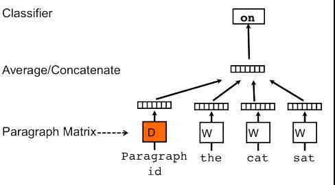
因此 doc2vec 就是在 word2vec 多加了一层向量。
30.1 paper
# dir.create("figure")
readr::read_lines("../../emotion_detection_2019_ncov/analysis/doc2vec.Rmd") %>%
    str_subset("knitr::include_graphics") %>%
    str_extract("figure/.+\\.png") %>%
    map( ~ file.path(dirname(
        dirname("../../emotion_detection_2019_ncov/analysis/doc2vec.Rmd")
    ), .)) %>%
    # map(file.exists)
    map(file_copy, overwrite = TRUE, new_path = "figure/")
## [[1]]
## figure/para_id.png
##
## [[2]]
## figure/PV-BDOW.png文章可以参考 1405.4053v2.pdf
Our technique is inspired by the recent work in learning vector representations of words using neural networks (Bengio et al., 2006; Collobert & Weston, 2008; Mnih & Hinton, 2008; Turian et al., 2010; Mikolov et al., 2013a;c). In their formulation, each word is represented by a vector which is concatenated or averaged with other word vectors in a context, and the resulting vector is used to predict other words in the context.
这一段描述 CBOW 的做法,合并(row_stack)和求平均(Ave Pooling)是代码上具体的实现。
In our Paragraph Vector framework (see Figure 2), every paragraph is mapped to a unique vector, represented by a column in matrix \(D\) and every word is also mapped to a unique vector, represented by a column in matrix \(W\). The paragraph vector and word vectors are averaged or concatenated to predict the next word in a context. In the experiments, we use concatenation as the method to combine the Vectors.
就是加上 Para Id 的向量。
The paragraph token can be thought of as another word. It acts as a memory that remembers what is missing from the current context – or the topic of the paragraph. For this reason, we often call this model the Distributed Memory Model of Paragraph Vectors (PV-DM).
Para Id 衡量了一个句子的含义或者主题,是 Id Embedding。
The contexts are fixed-length and sampled from a sliding window over the paragraph. The paragraph vector is shared across all contexts generated from the same paragraph but not across paragraphs. The word vector matrix W, however, is shared across paragraphs. I.e., the vector for “powerful” is the same for all paragraphs.
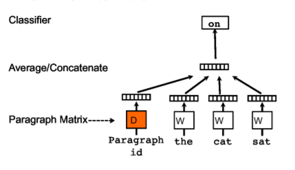
Figure 30.1: 这个理解非常地道。 Word2Vec 是需要滑动窗口的,保持长度一样。 对于同一个 Para 会滑动多出个输入 List。 Para Id 会跟随同一个 Para 产生的这些 List。 因此 Para Id 体现了 Para 本身的主题性。另外词向量是针对于所有 Para 参数共享的,每个 mini-batch 梯度下降都影响。 但是 Para Id 不会,是 Id Embedding,属于某一个 Para。
In summary, the algorithm itself has two key stages: 1 ) training to get word vectors \(W\), softmax weights \(U, b\) and paragraph vectors \(D\) on already seen paragraphs; and 2 ) “the inference stage” to get paragraph vectors \(D\) for new paragraphs (never seen before) by adding more columns in \(D\) and gradient descending on \(D\) while holding \(W, U, b\) fixed. We use \(D\) to make a prediction about some particular labels using a standard classifier, e.g., logistic regression.
突然看懂了,词向量、包括 softmax 的参数不动,把新的 Para 加入,进行梯度下降训练,拿到新的 D,就是 Para 的 Id Embedding 了。
Although the focus of this work is to represent texts, our method can be applied to learn representations for sequential data. In non-text domains where parsing is not available, we expect Paragraph Vector to be a strong alternative to bag-of-words and bag-of-n-grams models.
可以使用 doc2vec 进行序列特征的测试。
After being trained, the paragraph vectors can be used as features for the paragraph (e.g., in lieu of or in addition to bag-of-words). We can feed these features directly to conventional machine learning techniques such as logistic regression, support vector machines or K-means.
这样可以快速把 text data 转化为结构化数据,进行分析。
This model is also similar to the Skip-gram model in word vectors (Mikolov et al., 2013c).
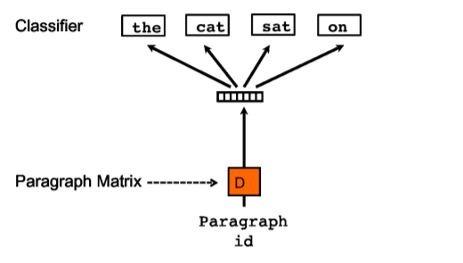
Figure 30.2: 这种情况就是反过来的 skip-gram 了。
In fact, paragraph vectors have the potential to overcome many weaknesses of bag-of-words models.
(???) 一直拿 doc2vec 和 BOW 对比,其实这里不是想要说和词向量比优劣,参考词向量的思路而已。 真正的目的是 BOW 是一个 text data 转结构化数据的方式,doc2vec 要去替代它,产生一个更可靠、End to End 的方式。
30.2 demo
# emotion_train=pd.read_csv(r'D:/JupyterNotebook/emotion/data/nCoV_100k_train.labled.csv')
# 用相对路径
emotion_train=pd.read_csv('../data/nCoV_100k_train.labled.csv')
stopwords = open('../data/cn_stopwords.txt',encoding='utf-8').read().split()
stopwords = frozenset(stopwords)
print(len(stopwords))746
| 微博id | 微博发布时间 | 发布人账号 | 微博中文内容 | 微博图片 | 微博视频 | 情感倾向 | |
|---|---|---|---|---|---|---|---|
| 99997 | 4473035904435920 | 02月17日 19:18 | 蝌蚪五线谱 | #微博辟谣#没有证据表明,吃大蒜、漱口水、涂抹芝麻油、生理盐水洗鼻子等手段可以防止感染新型冠… | [’https://ww4.sinaimg.cn/orj360/6d2cc4e6ly1gbz… | [] | 0 |
| 99998 | 4472950743017610 | 02月17日 13:40 | 医库 | 【新冠疫情最受关注的十一篇英文核心期刊论文全解析】本文整理了关于新型冠状病毒最受关注的十一篇… | [] | [] | 1 |
| 99999 | 4472870103356260 | 02月17日 08:19 | 有度为王 | 从蝙蝠携带的冠状病毒变异成2019-nCoV冠状病毒,怎样才能发生变异呢?有两种可能1.自然… | [] | [] | 0 |
def cut_sen(text):
    stop_list=[line[:-1] for line in open('../input/cn_stopwords.txt',encoding='utf-8')]
    result=[]
    for each in text:
        each_cut=jieba.cut(each)
        each_split=' '.join(each_cut).split()
        each_result=[word for word in each_split if word not in stop_list]
        result.append(' '.join(each_result))
return resultBuilding prefix dict from the default dictionary … Loading model from cache C:~1.cache Loading model cost 0.661 seconds. Prefix dict has been built succesfully.
[’[‘, "’", ‘写’, ’‘, ’年’]
改变成Doc2vec所需要的输入样本格式,由于gensim里Doc2vec模型需要的输入为固定格式, 输入样本为:[句子,句子序号],这里需要用gensim中Doc2vec里的TaggedDocument来包装输入的句子
def tagged(cut_sen):
    x_train=[]
    for k,v in enumerate(cut_sen):
        word_list=v.split(' ')
        l=len(word_list)
        word_list[l-1]=word_list[l-1].strip()
        documnet=TaggedDocument(word_list,tags=[k])
        x_train.append(documnet)

return x_train?TaggedDocument
用gensim里infer_vector()预测新的句子,这里根据经验,alpha(学习步长)设置小一些,迭代次数设置大一些。
找到训练样本中与这个句子最相近的10个句子。可以看到训练出来的结果与测试的新句子是有关联的。def train(tagged,size=300):
model=gensim.models.doc2vec.Doc2Vec(tagged,min_count=1,window=3,vector_size=size,sample=1e-3,workers=4)
model.train(tagged,total_examples=model.corpus_count,epochs=5)
return modelfor count,sim in sims:
print(count,sim)
sen=emotion_train['微博中文内容'][count]
words=''
for word in sen:
words=words+word+' '
print(words,sim,len(sen))4997 0.18822115659713745 【 上 海 药 物 所 、 武 汉 病 毒 所 联 合 发 现 : # 双 黄 连 可 抑 制 新 型 冠 状 病 毒 # 】 3 1 日 从 中 国 科 学 院 上 海 药 物 所 获 悉 , 该 所 和 武 汉 病 毒 所 联 合 研 究 初 步 发 现 , 中 成 药 # 双 黄 连 口 服 液 可 抑 制 新 型 冠 状 病 毒 # 。 此 前 , 上 海 药 物 所 启 动 由 蒋 华 良 院 士 牵 头 的 抗 新 型 冠 状 病 毒 感 染 肺 炎 药 物 研 究 应 急 攻 关 团 队 , 在 前 期 S A R S 相 关 研 究 和 药 物 发 现 成 ? 展 开 全 文 c 0.18822115659713745 151 2443 0.18802590668201447 # 张 定 宇 新 冠 肺 炎 是 自 限 性 疾 病 # 然 而 我 最 没 有 信 心 的 就 是 自 己 的 免 疫 力 。 青 霉 素 头 孢 都 过 敏 的 我 , 哺 乳 期 的 我 , 肥 宅 的 我 , 最 近 每 天 起 早 做 做 操 ( 上 学 时 候 学 过 的 第 十 三 套 广 播 体 操 ) 都 在 告 诉 自 己 , 这 是 保 命 操 , 加 油 ! 坚 持 ! ? 0.18802590668201447 101 1907 0.1783551424741745 / / @ 金 曲 唱 不 停 : # 王 晨 艺 繁 华 声 # 果 然 , 晨 艺 还 是 属 于 舞 者 的 舞 台 , 只 有 在 那 里 他 才 能 尽 情 的 发 光 发 热 , 享 受 聚 光 灯 下 的 每 一 刻 。 继 续 加 油 吧 少 年 ! # 舞 蹈 风 暴 首 播 # L 湖 南 卫 视 舞 蹈 风 暴 的 微 博 视 频 ? ? ? 0.1783551424741745 92 2014 0.17595165967941284 / / @ 蔡 徐 坤 你 翻 不 翻 我 牌 : k k / / @ A A A 大 笨 猫 : ? ? ? ? ? ? / / @ K S t a r a i n : ? ? ? ? / / @ 春 光 灿 烂 桔 八 戒 : 扩 / / @ 展 台 手 册 : 看 看 汉 口 医 院 看 看 汉 口 医 院 因 为 是 小 医 院 所 以 没 有 什 么 人 看 到 但 是 是 【 第 一 个 】 接 收 发 热 病 人 的 医 院 啊 ! 这 样 下 去 不 是 办 法 啊 ! ! 0.17595165967941284 124 1966 0.17409856617450714 【 买 感 冒 药 先 看 舌 苔 】 1 . 风 寒 型 感 冒 : 舌 苔 白 , 伴 有 面 色 发 白 、 恶 寒 重 、 发 热 轻 或 不 发 热 。 2 . 风 热 型 感 冒 : 舌 苔 黄 或 微 白 , 伴 有 恶 寒 轻 。 3 . 暑 湿 型 感 冒 : 舌 苔 黄 、 厚 、 腻 , 伴 有 恶 寒 发 热 。 ? 0.17409856617450714 86
[[False, False, False], [False, False, False], [False, False, False]]
False
30.3 扩展
参考 https://stackoverflow.com/questions/42781292/doc2vec-get-most-similar-documents
documents = [TaggedDocument(doc, [i]) for i, doc in enumerate(text_splited_list)]
model = Doc2Vec(documents, vector_size=5, window=10, min_count=1, workers=4, epochs = 100)tokens = "下一步考虑在很多模型里面替换 LSTM 为 GRU。或者一起使用"
tokens = [word_item for word_item in jieba.cut(tokens) if word_item not in stopwords]
new_vector = model.infer_vector(tokens)
# Find the top-N most similar docvecs from the training set.
sims = model.docvecs.most_similar([new_vector], topn =100)
most_sim_sent_list = [i for i,j in sims]
most_sim_sent_list
text.iloc[most_sim_sent_list]31 动态词向量
Combining dynamic topic models and dynamic word embeddings is an area for future study. (Rudolph and Blei 2017)
可以理解,DTM (DTM)和DWE两个NLP算法是有共同的。
In this section, we review Bernoulli embeddings for text and show how to include dynamics into the model. (Rudolph and Blei 2017) Dynamic Bernoulli embeddings. Dynamic Bernoulli embeddings extend Bernoulli embeddings to text data over time. (Rudolph and Blei 2017)
这是这篇文献的贡献,完成动态在模型上的实现。
We then derive the objective function for dynamic embeddings and develop stochastic gradients to optimize it. (Rudolph and Blei 2017)
也是使用传统的梯度下降完成。
Context vectors are shared across all positions in the text but the embedding vectors are only shared within a time slice. (Rudolph and Blei 2017) Graphical representation of a dynamic embedding for text data in \(T\) time slices, \(X^{(1)}, \cdots, X^{(T)} .\) The embedding vectors \(\rho_{v}\) of each term evolve over time. The context vectors are shared across all time slices. (Rudolph and Blei 2017)
因此文本向量是共享全文的,但是词向量是每个时间切片上独立存在,这样就清楚了,也就是说因为词向量是在每个时间切片上独立训练,因此可以看到词向量的变化。 这样理解下来,DWE 模型其实和 DTM 类似,就是各个时间切片上做相对独立的模型,没有太复杂的算法。
32 词向量训练的经验
1.5万样本还可以
- 太少,词向量太差
- 太多,太泛化了 ,不能体现这个样本的独特性
附录
参考文献
33 Wide&Deep
- one-hot 就是 wide
- embedding 就是 deep
附录
33.1 jieba 分词
33.2 Pattern 包的兼容问题
一直是这个报错。
i guess i found the solution i have been trying to install pattern, but its production stopped some how and it is the source of the problem. https://github.com/RaRe-Technologies/gensim/issues/2216
参考 https://github.com/RaRe-Technologies/gensim/issues/2216#issuecomment-653650047
pattern 是 Python 2.6,是一个黑洞。
33.3 金融报告情感分析和股价波动
思路上的贡献是 Prince Kumar (2019) 对标题、第一段、最后一段进行情感分打分,也是调用预训练词典,然后用三个情感分对股价进行预测。我目前在想,如果我们的情感分预测会有偏差、大批量跑不出来,可以采用他的思路。
- 对标题、第一段、最后一段进行情感分打分,这样结果可以分批出来
- 不需要整篇新闻进行训练,减少数据处理
- Prince Kumar (2019) 增加了
Combined字段是整合标题、第一段、最后一段出情感分,防止了对标题、第一段、最后一段的选择带来的误差。 - Prince Kumar (2019) 也是做解释性研究,而非预测,所以他的思想可以借鉴。
情感分效果, Prince Kumar (2019) 进行了
- 1天、5天、30天股价波动比较
- 两种不同词典的情感分效果对比
- 整体和标题、第一段、最后一段的情感分效果进行对比
一共 3x2x2=12个回归结果。
## [1] 568 24cat_ft <- function(x) {
case_when(x > .02 ~ "Increase",
x < -.02 ~ "Decrease",
TRUE ~ "No_Change")
}
df <-
df %>%
select(starts_with("Per_Change_T")) %>%
mutate_all(cat_ft) %>%
`names<-`(paste0("Class", c(1, 5, 30))) %>%
bind_cols(df)fun <- function(stri) {
as.integer(gsub(" ", "", gsub("d", "", gsub(
"a", "", substr(stri, 1, 4)
))))
}
df$Delta <- fun(df$TimeDelta)library(caret)
set.seed(1995)
tetr <- createDataPartition(df$Per_Change_T1, p = .75, list = F)
tr <- df[tetr, ]
te <- df[-tetr, ]run_model <-
function(tr, y = "Per_Change_T1", te, x_scope = "Finance", is_combine = FALSE) {
if (isFALSE(is_combine)) {
is_x_scope <- FALSE
is_combine_condition<- TRUE
} else {
is_x_scope <- TRUE
is_combine_condition<- FALSE
}
tr_ft_list <-
tr %>%
names() %>%
str_subset(x_scope, negate = is_x_scope) %>%
str_subset("Combined", negate = is_combine_condition) %>%
c(y, "mkvaltq", "Delta")
tr_input <-
tr %>%
select(tr_ft_list)
mod_form <- as.formula(glue::glue("{y} ~ ."))
mod <- lm(mod_form, data = tr_input)
beta_df <- broom::tidy(mod) %>%
select(term, estimate, p.value)
# browser()
rmse <- sqrt(mean(te[[y]] - predict(mod, newdata=te)^2))
return(list(mod, beta_df, rmse))
}for (is_combine1 in c(FALSE, TRUE)) {
for (i in y_list) {
list(
run_model(tr, i, te, x_scope = "Finance", is_combine = is_combine1)[2],
run_model(tr, i, te, x_scope = "General", is_combine = is_combine1)[2]
) %>%
knitr::kable() %>%
print()
# debugonce(run_model)
run_model(tr, i, te, x_scope = "Finance", is_combine = is_combine1)[3] %>% paste0('RMSE(1): ', .) %>% print()
run_model(tr, i, te, x_scope = "General", is_combine = is_combine1)[3] %>% paste0('RMSE(2): ', .) %>% print()
}
}
|
|
[1] “RMSE(1): 0.0510154637879535” [1] “RMSE(2): 0.0508017869059139”
|
|
[1] “RMSE(1): 0.0501008019420093” [1] “RMSE(2): 0.04973462738712”
|
|
[1] “RMSE(1): 0.140961679744847” [1] “RMSE(2): 0.14098262123184”
|
|
[1] “RMSE(1): 0.0509200459409371” [1] “RMSE(2): 0.051054993288609”
|
|
[1] “RMSE(1): 0.050156098280063” [1] “RMSE(2): 0.050358381850046”
|
|
[1] “RMSE(1): 0.141038659217749” [1] “RMSE(2): 0.14103797712882”
33.4 Word Movers’ Distance
参考 gensim: Word Movers’ Distance
WMD enables us to assess the “distance” between two documents in a meaningful way, even when they have no words in common. It uses word2vec [4] vector embeddings of words. It been shown to outperform many of the state-of-the-art methods in k-nearest neighbors classification [3].
算句子之间的距离。
33.5 mask 使用
mask = keras.layers.Masking(mask_value=0, input_shape=(time_step,feature_size))(input)参考 Masking and padding with Keras | TensorFlow Core 和 海晨威 (2020)
“Masking” is how layers are able to know when to skip / ignore certain timesteps in sequence inputs.
虽然是 padding 上去的,但是要让模型知道。
33.6 自定义下载 nltk 数据
会报错,因为网络访问不了。 手动下载时
中间要定义corpora,再放入stopwords
D:\install\miniconda\nltk_data\corpora\stopwords
D:\install\miniconda\nltk_data\stopwords
参考文献
Axelbrooke, Stuart. 2015. “LDA Alpha and Beta Parameters - the Intuition.” Thought Vector Blog. 2015. https://www.thoughtvector.io/blog/lda-alpha-and-beta-parameters-the-intuition/.
Ayyadevara, V Kishore. 2018. Pro Machine Learning Algorithms: A Hands-on Approach to Implementing Algorithms in Python and R. Apress.
Blei, David M., and John D. Lafferty. 2006. “Dynamic Topic Models.” In Machine Learning, Proceedings of the Twenty-Third International Conference (Icml 2006), Pittsburgh, Pennsylvania, Usa, June 25-29, 2006.
Blei, David M, Andrew Y Ng, and Michael I Jordan. 2003. “Latent Dirichlet Allocation.” Journal of Machine Learning Research 3 (Jan): 993–1022.
Cai-Pincus, Jingfei. 2017. “PMC-Text-Mining: The Aim of This Project Is to Use the Text from Biomedical and Life Science Literature to Gain Insights on Research Topic Trends over Time.” GitHub. 2017. https://github.com/Ailuropoda1864/PMC-text-mining.
Clark, Stephen, and Mark Gales. 2013. “Topic Modelling and Latent Dirichlet Allocation.” add2bibtex. 2013. https://www.cl.cam.ac.uk/teaching/1213/L101/clark_lectures/lect7.pdf.
Ganesan, Kavita. 2020. “Gensim Word2vec Tutorial – Full Working Example.” Kavita Ganesan. 2020. https://kavita-ganesan.com/gensim-word2vec-tutorial-starter-code/.
Griffiths, Thomas L, and Mark Steyvers. 2004. “Finding Scientific Topics.” Proceedings of the National Academy of Sciences 101 (suppl 1): 5228–35.
Jameel, Shoaib, and Wai Lam. 2013. “A Nonparametric N-Gram Topic Model with Interpretable Latent Topics.” In Information Retrieval Technology, edited by Rafael E. Banchs, Fabrizio Silvestri, Tie-Yan Liu, Min Zhang, Sheng Gao, and Jun Lang, 74–85. Berlin, Heidelberg: Springer Berlin Heidelberg.
Ledolter, Johannes. 2013. Data Mining and Business Analytics with R. 1st ed. Wiley.
Liu, Ethen. 2015. “Latent Dirichlet Allocation Using Gibbs Sampling.” ethen8181/machine-learning. 2015. https://ethen8181.github.io/machine-learning/clustering_old/topic_model/LDA.html.
Mikolov, Tomas, Ilya Sutskever, Kai Chen, Greg Corrado, and Jeffrey Dean. 2013. “Distributed Representations of Words and Phrases and Their Compositionality.” CoRR abs/1310.4546. http://arxiv.org/abs/1310.4546.
Oleinikov, Pavel. 2019. “Topic Modeling in R.” DataCamp. 2019. https://www.datacamp.com/courses/topic-modeling-in-r.
Phan, Xuan-Hieu, Le-Minh Nguyen, and Susumu Horiguchi. 2008. “Learning to Classify Short and Sparse Text & Web with Hidden Topics from Large-Scale Data Collections.” In Proceedings of the 17th International Conference on World Wide Web, 91–100.
Pleplé, Quentin. 2013. “Perplexity to Evaluate Topic Models.” Self-Published. 2013. http://qpleple.com/perplexity-to-evaluate-topic-models/.
Prabhakaran, Selva. 2020. “Topic Modeling with Gensim (Python).” add2bibtex. 2020. https://github.com/JiaxiangBU/add2bibtex.
Prevos, Peter. 2018. “Defining Marketing with the Rvest and Tidytext Packages.” The Lucid Manager. 2018. https://lucidmanager.org/rvest-and-tidytext/.
Prince Kumar, Amratansh Sharma, Simon Jones. 2019. “Stock-Price-Predictions.” GitHub. 2019. https://github.com/amratansh/Stock-Price-Predictions.
Rudolph, Maja, and David Blei. 2017. “Dynamic Bernoulli Embeddings for Language Evolution.” http://arxiv.org/abs/1703.08052.
Řehůřek, Radim. 2014. “Word2vec Tutorial.” RaRe Technologies. 2014. https://rare-technologies.com/word2vec-tutorial/.
Shperber, Gidi. 2019. “Doc2Vec的一个轻量级介绍.” 小小挖掘机. 2019. https://mp.weixin.qq.com/s/mhahB9zt6vEMWn7SFqXzeQ.
Shrivarsheni. 2020. “101 Nlp Exercises (Using Modern Libraries).” Machine Learning Plus. 2020. https://www.machinelearningplus.com/nlp/nlp-exercises/.
Silge, Julia, and David Robinson. 2019. “Text Mining with R: A Tidy Approach.” bookdown. 2019. https://www.tidytextmining.com/topicmodeling.html.
Svitlana. 2019. “Dtmvisual: This Package Consists of Functionalities for Dynamic Topic Modelling and Its Visualization.” GitHub. 2019. https://github.com/GSukr/dtmvisual.
Wang, Zhongdao, Liang Zheng, Yali Li, and Shengjin Wang. 2019. “Linkage Based Face Clustering via Graph Convolution Network.”
张佩瑶, and 刘东苏. 2019. “基于词向量和BTM的短文本话题演化分析.” 数据分析与知识发现, no. 3: 95–101.
张志飞, 苗夺谦, and 高灿. 2013. “基于 Lda 主题模型的短文本分类方法.” 计算机应用 33 (06): 1587–90.
海晨威. 2020. “NLP中各框架对变长序列的处理全解.” PaperWeekly. 2020. https://mp.weixin.qq.com/s/KxgA1U-mh9Tc1J1T9Aedrw.
葫芦娃. 2018. 百面机器学习.