learn_nlp
可视化NLP的结果
Jiaxiang Li 2019-03-07
之前使用 Keras 训练的 NLP 小例子 ,有一个技能没有训练。 里面的词向量是已经训练好了,重点是模型,这个例子,介绍了词向量的构建方式。
可以发现大部分的文字都没有学习和识别,这也是证明了一个Xgboost 加上简单的词效果不好。
参考 Blog
knitr::opts_chunk$set(warning = FALSE, message = FALSE)
# data wrangling
library(tidyverse)
library(readr)

# plotting
library(ggthemes)
theme_set(theme_minimal())

# text prep
library(text2vec)

# ml
library(caret)
library(xgboost)

# explanation
library(lime)
数据来自 www.kaggle.com
unzip("datasets/womens-ecommerce-clothing-reviews.zip", exdir = 'datasets')
解压数据。
clothing_reviews_raw <- read_csv("datasets/Womens Clothing E-Commerce Reviews.csv")
clothing_reviews_raw %>% head
## # A tibble: 6 x 11
##      X1 `Clothing ID`   Age Title `Review Text` Rating `Recommended IN~
##   <dbl>         <dbl> <dbl> <chr> <chr>          <dbl>            <dbl>
## 1     0           767    33 <NA>  Absolutely w~      4                1
## 2     1          1080    34 <NA>  "Love this d~      5                1
## 3     2          1077    60 Some~ I had such h~      3                0
## 4     3          1049    50 My f~ I love, love~      5                1
## 5     4           847    47 Flat~ This shirt i~      5                1
## 6     5          1080    49 Not ~ I love tracy~      2                0
## # ... with 4 more variables: `Positive Feedback Count` <dbl>, `Division
## #   Name` <chr>, `Department Name` <chr>, `Class Name` <chr>
clothing_reviews <-
    clothing_reviews_raw %>%
    mutate(Liked = as.factor(ifelse(Rating == 5, 1, 0)),
           text = paste(Title, `Review Text`),
           text = gsub("NA", "", text))
把评论标题和文本合并成一段文字。
glimpse(clothing_reviews)
## Observations: 23,486
## Variables: 13
## $ X1                        <dbl> 0, 1, 2, 3, 4, 5, 6, 7, 8, 9, 10, 11...
## $ `Clothing ID`             <dbl> 767, 1080, 1077, 1049, 847, 1080, 85...
## $ Age                       <dbl> 33, 34, 60, 50, 47, 49, 39, 39, 24, ...
## $ Title                     <chr> NA, NA, "Some major design flaws", "...
## $ `Review Text`             <chr> "Absolutely wonderful - silky and se...
## $ Rating                    <dbl> 4, 5, 3, 5, 5, 2, 5, 4, 5, 5, 3, 5, ...
## $ `Recommended IND`         <dbl> 1, 1, 0, 1, 1, 0, 1, 1, 1, 1, 0, 1, ...
## $ `Positive Feedback Count` <dbl> 0, 4, 0, 0, 6, 4, 1, 4, 0, 0, 14, 2,...
## $ `Division Name`           <chr> "Initmates", "General", "General", "...
## $ `Department Name`         <chr> "Intimate", "Dresses", "Dresses", "B...
## $ `Class Name`              <chr> "Intimates", "Dresses", "Dresses", "...
## $ Liked                     <fct> 0, 1, 0, 1, 1, 0, 1, 0, 1, 1, 0, 1, ...
## $ text                      <chr> " Absolutely wonderful - silky and s...
clothing_reviews %>%
    ggplot(aes(x = Liked, fill = Liked)) +
    geom_bar(alpha = 0.8) +
    # scale_fill_tableau(palette = "tableau20") +
    guides(fill = FALSE)
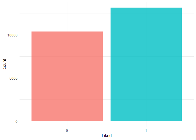
查看好评的差异,没有不平衡问题。
todo 可以参考 ranking data analysis 做多分类分析。
set.seed(42)
idx <- createDataPartition(clothing_reviews$Liked,
                           p = 0.8,
                           list = FALSE,
                           times = 1)

clothing_reviews_train <- clothing_reviews[ idx,]
clothing_reviews_test  <- clothing_reviews[-idx,]
引入 caret 的目的。
get_matrix <- function(text) {
  it <- itoken(text, progressbar = FALSE)
  create_dtm(it, vectorizer = hash_vectorizer())
}
建立产生词向量的函数。
clothing_reviews_train %>% dim
## [1] 18789 13
clothing_reviews_test %>% dim
## [1] 4697 13
训练集只有2万不到的样本。
dtm_train <- get_matrix(clothing_reviews_train$text)
str(dtm_train)
## Formal class 'dgCMatrix' [package "Matrix"] with 6 slots
##   ..@ i       : int [1:889012] 304 764 786 788 793 794 1228 2799 2819 3041 ...
##   ..@ p       : int [1:262145] 0 0 0 0 0 0 0 0 0 0 ...
##   ..@ Dim     : int [1:2] 18789 262144
##   ..@ Dimnames:List of 2
##   .. ..$ : chr [1:18789] "1" "2" "3" "4" ...
##   .. ..$ : NULL
##   ..@ x       : num [1:889012] 1 1 2 1 2 1 1 1 1 1 ...
##   ..@ factors : list()
dtm_test <- get_matrix(clothing_reviews_test$text)
str(dtm_test)
## Formal class 'dgCMatrix' [package "Matrix"] with 6 slots
##   ..@ i       : int [1:222314] 2793 400 477 622 2818 2997 3000 4500 3524 2496 ...
##   ..@ p       : int [1:262145] 0 0 0 0 0 0 0 0 0 0 ...
##   ..@ Dim     : int [1:2] 4697 262144
##   ..@ Dimnames:List of 2
##   .. ..$ : chr [1:4697] "1" "2" "3" "4" ...
##   .. ..$ : NULL
##   ..@ x       : num [1:222314] 1 1 1 1 1 1 1 1 1 1 ...
##   ..@ factors : list()
xgb_model <- xgb.train(list(max_depth = 7,
                            eta = 0.1,
                            objective = "binary:logistic",
                            eval_metric = "error", nthread = 1),
                       xgb.DMatrix(dtm_train,
                                   label = clothing_reviews_train$Liked == "1"),
                       nrounds = 50)
建立一个 Xgboost 模型。
pred <- predict(xgb_model, dtm_test)

confusionMatrix(clothing_reviews_test$Liked,
                as.factor(round(pred, digits = 0)))
## Confusion Matrix and Statistics
##
##           Reference
## Prediction    0    1
##          0 1370  701
##          1  421 2205
##
##                Accuracy : 0.7611
##                  95% CI : (0.7487, 0.7733)
##     No Information Rate : 0.6187
##     P-Value [Acc > NIR] : < 2.2e-16
##
##                   Kappa : 0.5085
##  Mcnemar's Test P-Value : < 2.2e-16
##
##             Sensitivity : 0.7649
##             Specificity : 0.7588
##          Pos Pred Value : 0.6615
##          Neg Pred Value : 0.8397
##              Prevalence : 0.3813
##          Detection Rate : 0.2917
##    Detection Prevalence : 0.4409
##       Balanced Accuracy : 0.7619
##
##        'Positive' Class : 0
##
confusionMatrix很快速的给出多个指标,非常方便。
todo 做中文的
explainer <- lime(clothing_reviews_train$text,
                  xgb_model,
                  preprocess = get_matrix)
interactive_text_explanations(explainer)
会产生一个 Shiny Apps,具体可以查看 Blog
explanations <- lime::explain(clothing_reviews_test$text[1:4], explainer, n_labels = 1, n_features = 5)
plot_text_explanations(explanations)
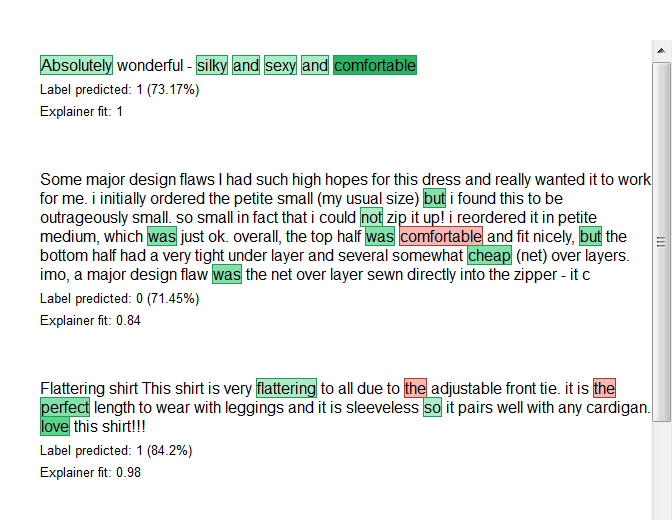
这里显示了哪些词是正向作用,那些是负向作用。
plot_features(explanations)
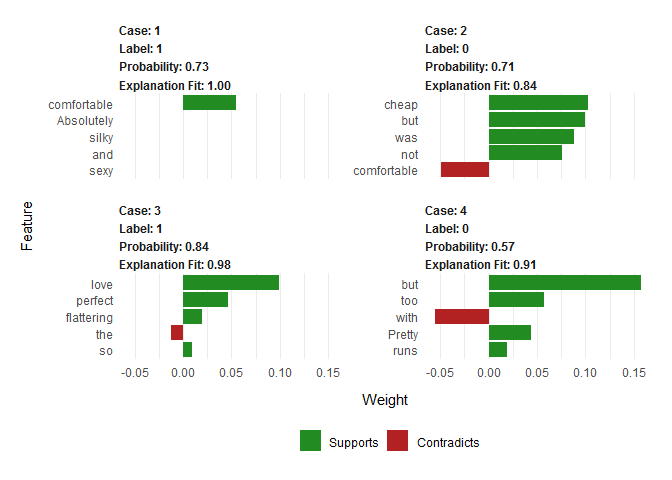
这里体现了具体一个 case 中每个变量的贡献程度。
这也解释了为什么一些模型结果是先反馈结果,成为一列,再反馈这个结果的概率是多少。 这也是一种反馈的范式。