1 floor 到每周处理方法

参考 Reback (2017) 和 Leung (2018)

time_column = pd.to_datetime(df2['time'])
time_column = time_column.dt.to_period("W").dt.to_timestamp()

如果使用 pd.Series.dt.floor("M") 会产生报错ValueError: <MonthEnd> is a non-fixed frequency。

例如，

import pandas as pd
import numpy as np
import scipy.sparse as sparse

#import sparse matrix
sp=sparse.load_npz('../output/sp.npz')
score=sp.todense()

score.__class__

numpy.matrix

df1 = pd.DataFrame(score)

df1.head()

	0	1	4	5	6	7	8	9	10	11	12	14
0	0.115958	0.000000	0.000000	0.059606	0.011118	0.382871	0.022741	0.000000	0.000000	0.036845	0.059429	0.311433
1	0.707055	0.000000	0.016321	0.000000	0.000000	0.000000	0.000000	0.000000	0.000000	0.000000	0.072367	0.204257
2	0.000000	0.000000	0.139806	0.000000	0.000000	0.128367	0.000000	0.000000	0.288471	0.418322	0.000000	0.025034
3	0.012516	0.000000	0.136892	0.000000	0.000000	0.284297	0.000000	0.036387	0.000000	0.135912	0.000000	0.393996
4	0.000000	0.013008	0.000000	0.000000	0.000000	0.024693	0.000000	0.039126	0.000000	0.906986	0.000000	0.016187

score.shape

(133201, 15)

#import time series
df2 = pd.read_csv('../data/df_japan.csv',header=None,encoding='gbk',names=['time','none','catagory','title','content'])

df2.head()

	time	none	catagory	title	content
0	1946.05.15	3.0	NaN	苏评论家马西努著论痛斥阎锡山勾结日寇美军帮助日阎进攻解放区，不符莫斯科三国决议	痛斥阎锡山勾结日寇美军帮助日阎进攻解放区，不符莫斯科三国决议【新华社延安十二日电】莫斯科广播…
1	1946.05.15	3.0	NaN	片山组阁搁浅日共力主联合内阁	日共力主联合内阁【新华社延安十二日电】东京讯：日本社会党领导人，日来与日共谈判组织新阁问题，…
2	1946.05.15	4.0	NaN	五月杂感	张香山一到日历翻掀到五月，总感到有些沉重，那种触目惊心的流血，暴虐耻辱的日子，实在太多了——…
3	1946.05.16	1.0	NaN	苏皖冀晋鲁豫各地战云密布国民党策动全面内战倾两师之众进迫我定远县境兖州伪逆吴化文部二千余出犯被击退	国民党策动全面内战倾两师之众进迫我定远县境兖州伪逆吴化文部二千余出犯被击退【新华社延安十三日…
4	1946.05.16	2.0	NaN	今日的“丛台”记边区卫生局流诊所	记边区卫生局流诊所邯郸城厢东北角的“丛台”，据说是战国时代赵武灵王的遗址。为了这几个小土阜和…

time_column = pd.to_datetime(df2['time'])
time_column = time_column.dt.to_period("W").dt.to_timestamp()

time_column.shape

(133201,)

df3 = pd.concat([time_column, df1], axis=1)

df3.head()

	time	0	1	4	5	6	7	8	9	10	11	12	14
0	1946-05-13	0.115958	0.000000	0.000000	0.059606	0.011118	0.382871	0.022741	0.000000	0.000000	0.036845	0.059429	0.311433
1	1946-05-13	0.707055	0.000000	0.016321	0.000000	0.000000	0.000000	0.000000	0.000000	0.000000	0.000000	0.072367	0.204257
2	1946-05-13	0.000000	0.000000	0.139806	0.000000	0.000000	0.128367	0.000000	0.000000	0.288471	0.418322	0.000000	0.025034
3	1946-05-13	0.012516	0.000000	0.136892	0.000000	0.000000	0.284297	0.000000	0.036387	0.000000	0.135912	0.000000	0.393996
4	1946-05-13	0.000000	0.013008	0.000000	0.000000	0.000000	0.024693	0.000000	0.039126	0.000000	0.906986	0.000000	0.016187

df4 = df3.groupby(['time']).agg('mean')

df4.shape

(3823, 15)

df4.to_csv("../output/LDA_score_with_weekly_time.csv", index=False)

2 groupby

参考易执 (2020)

# default_exp groupby

# export
import pandas as pd
import numpy as np

#export
def build_data():
    
    np.random.seed(100)
    company=["A","B","C"]

    data=pd.DataFrame({
        "company":[company[x] for x in np.random.randint(0,len(company),10)],
        "salary":np.random.randint(5,50,10),
        "age":np.random.randint(15,50,10)
    }
    )

#export
data

	company	salary	age
0	A	19	17
1	A	39	42
2	A	29	19
3	C	20	46
4	C	41	16
5	A	48	28
6	C	21	34
7	B	14	19
8	C	34	42
9	C	27	18

group = data.groupby("company")

group.__class__

pandas.core.groupby.generic.DataFrameGroupBy

from pprint import pprint as p

p(list(group))

[(‘A’, company salary age 0 A 19 17 1 A 39 42 2 A 29 19 5 A 48 28), (‘B’, company salary age 7 B 14 19), (‘C’, company salary age 3 C 20 46 4 C 41 16 6 C 21 34 8 C 34 42 9 C 27 18)]

# export
# 多个字段进行汇总
def dplyr_summarize(group, agg_func = 'mean'):
    return group.agg(agg_func)

dplyr_summarize(group, 'mean')

	salary	age
company
A	33.75	26.5
B	14.00	19.0
C	28.60	31.2

# 或者用字典自定义
group.agg({"salary": "mean", "age": "median"})

	salary	age
company
A	33.75	23.5
B	14.00	19.0
C	28.60	34.0

dplyr_summarize(group, {"salary": "mean", "age": "median"})

	salary	age
company
A	33.75	23.5
B	14.00	19.0
C	28.60	34.0

这里 agg 相当于 dplyr::summarize，而transform 相当于 dplyr::mutate

#export
def dplyr_mutate(group, agg_func = 'mean'):
    return group.transform(agg_func)

dplyr_mutate(group, 'mean')

	salary	age
0	33.75	26.5
1	33.75	26.5
2	33.75	26.5
3	28.60	31.2
4	28.60	31.2
5	33.75	26.5
6	28.60	31.2
7	14.00	19.0
8	28.60	31.2
9	28.60	31.2

3 pandas 1.0.0

参考 https://dev.pandas.io/docs/whatsnew/v1.1.0.html

# !pip install --upgrade pandas==1.0.0rc0

import pandas as pd
pd.__version__

‘1.0.0rc0’

df = pd.DataFrame({
    'A': [1,2,3],
    'B': ['a','b','c'],
    'C': [False, True, False]
})

df.info()

<class ‘pandas.core.frame.DataFrame’> RangeIndex: 3 entries, 0 to 2 Data columns (total 3 columns): # Column Non-Null Count Dtype — —— ————– —– 0 A 3 non-null int64 1 B 3 non-null object 2 C 3 non-null bool
dtypes: bool(1), int64(1), object(1) memory usage: 179.0+ bytes

from pprint import pprint as p

p(df.to_markdown())

(‘| | A | B | C |’ ‘|—:|—-:|:—-|:——|’ ‘| 0 | 1 | a | False |’ ‘| 1 | 2 | b | True |’ ‘| 2 | 3 | c | False |’)

ImportError: Missing optional dependency 'tabulate'.  Use pip or conda to install tabulate.

# !pip install tabulate

参考 Datawhale (2020)

import pandas as pd
import numpy as np
print(pd.__version__)
print(np.__version__)

1.0.0rc0 1.17.4

4 import pandas series

arr = [0, 1, 2, 3, 4]
df = pd.Series(arr) # 如果不指定索引，则默认从 0 开始
df

0 0 1 1 2 2 3 3 4 4 dtype: int64

d = {'a':[1,2],'b':[2,3],'c':[3,4],'d':[4,5],'e':[5,6]}
df = pd.Series(d)
df

a [1, 2] b [2, 3] c [3, 4] d [4, 5] e [5, 6] dtype: object

df['a'][0]

1

5 cut number

df = pd.DataFrame({'A': [1,2,11,11,33,34,35,40,79,99], 
                   'B': [1,2,11,11,33,34,35,40,79,99]})
print(df)
df1 = df.groupby(pd.cut(df['A'], np.arange(0, 101, 10)))['B'].sum()
print(df1)

A B 0 1 1 1 2 2 2 11 11 3 11 11 4 33 33 5 34 34 6 35 35 7 40 40 8 79 79 9 99 99 A (0, 10] 3 (10, 20] 22 (20, 30] 0 (30, 40] 142 (40, 50] 0 (50, 60] 0 (60, 70] 0 (70, 80] 79 (80, 90] 0 (90, 100] 99 Name: B, dtype: int64

6 plot

df = pd.DataFrame({"revenue":[57,68,63,71,72,90,80,62,59,51,47,52],
                   "advertising":[2.1,1.9,2.7,3.0,3.6,3.2,2.7,2.4,1.8,1.6,1.3,1.9],
                   "month":range(1,13)})

ax = df.plot.bar("month", "revenue", color = "green")
df.plot.line("month", "advertising", secondary_y = True, ax = ax)
ax.set_xlim((-1,12));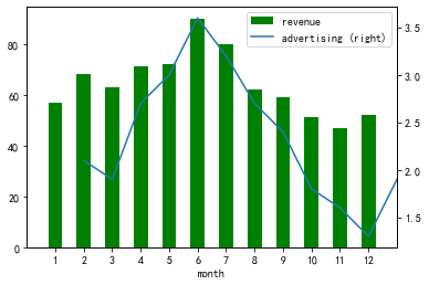

png

7 groupby 看统计结果

参考 Friedman (2020) describe().unstack()

# Import stats module
from scipy import stats

# Compute average age just below and above the threshold
era_900_1100 = df.loc[(df['expected_recovery_amount']<1100) & 
                      (df['expected_recovery_amount']>=900)]
by_recovery_strategy = era_900_1100.groupby(['recovery_strategy'])

era_900_1100.head()

	id	expected_recovery_amount	actual_recovery_amount	recovery_strategy	age	sex
158	520	900	504.790	Level 0 Recovery	34	Male
159	1036	900	539.535	Level 0 Recovery	34	Female
160	1383	900	554.745	Level 0 Recovery	24	Male
161	998	901	887.005	Level 0 Recovery	32	Male
162	1351	903	667.035	Level 0 Recovery	28	Male

by_recovery_strategy['age'].describe().unstack()

 recovery_strategy
count  Level 0 Recovery     89.000000
       Level 1 Recovery     94.000000
mean   Level 0 Recovery     27.224719
       Level 1 Recovery     28.755319
std    Level 0 Recovery      6.399135
       Level 1 Recovery      5.859807
min    Level 0 Recovery     18.000000
       Level 1 Recovery     18.000000
25%    Level 0 Recovery     23.000000
       Level 1 Recovery     24.000000
50%    Level 0 Recovery     26.000000
       Level 1 Recovery     29.000000
75%    Level 0 Recovery     31.000000
       Level 1 Recovery     33.000000
max    Level 0 Recovery     56.000000
       Level 1 Recovery     43.000000
dtype: float64

8 插入新行

参考 https://mp.weixin.qq.com/s/DS36kseh4hLW7i6hG_wwAA

import pandas as pd
df = pd.DataFrame({'a': [1,2], 'b': [3,4]})
print(df)

##    a  b
## 0  1  3
## 1  2  4

df.loc[1] = [5,6]
print(df)

##    a  b
## 0  1  3
## 1  5  6

9 loc 用数字 index

参考 https://mp.weixin.qq.com/s/DS36kseh4hLW7i6hG_wwAA

import pandas as pd
import numpy as np
data = {'animal': ['cat', 'cat', 'snake', 'dog', 'dog', 'cat', 'snake', 'cat', 'dog', 'dog'],
        'age': [2.5, 3, 0.5, np.nan, 5, 2, 4.5, np.nan, 7, 3],
        'visits': [1, 3, 2, 3, 2, 3, 1, 1, 2, 1],
        'priority': ['yes', 'yes', 'no', 'yes', 'no', 'no', 'no', 'yes', 'no', 'no']}

labels = ['a', 'b', 'c', 'd', 'e', 'f', 'g', 'h', 'i', 'j']

df = pd.DataFrame(data, index=labels)

df

	animal	age	visits	priority
a	cat	2.5	1	yes
b	cat	3.0	3	yes
c	snake	0.5	2	no
d	dog	NaN	3	yes
e	dog	5.0	2	no
f	cat	2.0	3	no
g	snake	4.5	1	no
h	cat	NaN	1	yes
i	dog	7.0	2	no
j	dog	3.0	1	no

df.loc[df.index[[3, 4, 8]], ['animal', 'age']]

	animal	age
d	dog	NaN
e	dog	5.0
i	dog	7.0

df.loc[[3, 4, 8], ['animal', 'age']]
KeyError: "None of [Int64Index([3, 4, 8], dtype='int64')] are in the [index]"

报错。

10 pandas 保存 zip

参考 Orac (2020)

import pandas as pd

df = pd.DataFrame(pd.np.random.randn(100,100))
df.to_csv('random_data.csv',index=False)

D:-packages_launcher.py:1: FutureWarning: The pandas.np module is deprecated and will be removed from pandas in a future version. Import numpy directly instead """Entry point for launching an IPython kernel.

!du -sh random_data.csv

196K random_data.csv

df.to_csv('random_data.gz', compression='gzip', index=False)

!du -sh random_data.gz

92K random_data.gz

df2 = pd.read_csv('random_data.gz')

df.shape,df2.shape

((100, 100), (100, 100))

11 文本直接相加

参考 https://stackoverflow.com/questions/19377969/combine-two-columns-of-text-in-dataframe-in-pandas-python

df['text01'] + '|' + df['text02']

12 `pd.to_datetime` 用 apply

参考 https://stackoverflow.com/questions/55460481/ignore-nan-values-when-searching-for-a-minimum-datetime

df['col1'].apply(pd.to_datetime).min()

而不要用

df['col1'] = pd.to_datetime(df['col1'])

这样设置一个中间变量的方式。

13 指定列 fillna

参考 https://stackoverflow.com/a/47315262

df.fillna({'a':0,'b':0})

14 groupby 怎么拿到 index

曲线救国

df.groupby('col1').size() # 就拿 index 了

15 reshape 1D to df

参考 https://stackoverflow.com/questions/36009907/numpy-reshape-1d-to-2d-array-with-1-column

reshape(-1, 1)

16 pull value from pandas df

参考 https://stackoverflow.com/a/47917648

df.loc[df.iata == 'PDX','name'].tolist()[0]

17 subset series by multiple index

参考 https://pandas.pydata.org/pandas-docs/stable/reference/api/pandas.Index.get_level_values.html

for text_part_names in text_part_names_list:
    sub_corpus = corpus.iloc[corpus.index.get_level_values(1) == text_part_names]
    print(sub_corpus.shape)

18 to_csv OSError

参考 https://stackoverflow.com/a/61242009

OSError: [Errno 22] Invalid argument

附录

18.1 棒球数据案例

参考 Venturi (2020)

18.1.1 The Statcast revolution

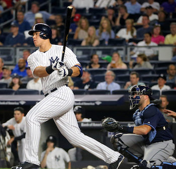
This is Aaron Judge. Judge is one of the physically largest players in Major League Baseball standing 6 feet 7 inches (2.01 m) tall and weighing 282 pounds (128 kg). He also hit the hardest home run ever recorded. How do we know this? Statcast.

Statcast is a state-of-the-art tracking system that uses high-resolution cameras and radar equipment to measure the precise location and movement of baseballs and baseball players. Introduced in 2015 to all 30 major league ballparks, Statcast data is revolutionizing the game. Teams are engaging in an “arms race” of data analysis, hiring analysts left and right in an attempt to gain an edge over their competition. This video describing the system is incredible.

In this notebook, we’re going to wrangle, analyze, and visualize Statcast data to compare Mr. Judge and another (extremely large) teammate of his. Let’s start by loading the data into our Notebook. There are two CSV files, judge.csv and stanton.csv, both of which contain Statcast data for 2015-2017. We’ll use pandas DataFrames to store this data. Let’s also load our data visualization libraries, matplotlib and seaborn.

import pandas as pd
import matplotlib.pyplot as plt
import seaborn as sns
%matplotlib inline

# Load Aaron Judge's Statcast data
judge = pd.read_csv('datasets/judge.csv')

# Load Giancarlo Stanton's Statcast data
stanton = pd.read_csv('datasets/stanton.csv')

18.1.2 What can Statcast measure?

The better question might be, what can’t Statcast measure?

Starting with the pitcher, Statcast can measure simple data points such as velocity. At the same time, Statcast digs a whole lot deeper, also measuring the release point and spin rate of every pitch.

Moving on to hitters, Statcast is capable of measuring the exit velocity, launch angle and vector of the ball as it comes off the bat. From there, Statcast can also track the hang time and projected distance that a ball travels.

Let’s inspect the last five rows of the judge DataFrame. You’ll see that each row represents one pitch thrown to a batter. You’ll also see that some columns have esoteric names. If these don’t make sense now, don’t worry. The relevant ones will be explained as necessary.

# Display all columns (pandas will collapse some columns if we don't set this option)
pd.set_option('display.max_columns', None)

# Display the last five rows of the Aaron Judge file
judge.tail()

	pitch_type	game_date	release_speed	release_pos_x	release_pos_z	player_name	batter	pitcher	events	description	spin_dir	spin_rate_deprecated	break_angle_deprecated	break_length_deprecated	zone	des	game_type	stand	p_throws	home_team	away_team	type	hit_location	bb_type	balls	strikes	game_year	pfx_x	pfx_z	plate_x	plate_z	on_3b	on_2b	on_1b	outs_when_up	inning	inning_topbot	hc_x	hc_y	tfs_deprecated	tfs_zulu_deprecated	pos2_person_id	umpire	sv_id	vx0	vy0	vz0	ax	ay	az	sz_top	sz_bot	hit_distance_sc	launch_speed	launch_angle	effective_speed	release_spin_rate	release_extension	game_pk	pos1_person_id	pos2_person_id.1	pos3_person_id	pos4_person_id	pos5_person_id	pos6_person_id	pos7_person_id	pos8_person_id	pos9_person_id	release_pos_y	estimated_ba_using_speedangle	estimated_woba_using_speedangle	woba_value	woba_denom	babip_value	iso_value	launch_speed_angle	at_bat_number	pitch_number
3431	CH	2016-08-13	85.6	-1.9659	5.9113	Aaron Judge	592450	542882	NaN	ball	NaN	NaN	NaN	NaN	14.0	NaN	R	R	R	NYY	TB	B	NaN	NaN	0	0	2016	-0.379108	0.370567	0.739	1.442	NaN	NaN	NaN	0	5	Bot	NaN	NaN	NaN	NaN	571912.0	NaN	160813_144259	6.960	-124.371	-4.756	-2.821	23.634	-30.220	3.93	1.82	NaN	NaN	NaN	84.459	1552.0	5.683	448611	542882.0	571912.0	543543.0	523253.0	446334.0	622110.0	545338.0	595281.0	543484.0	54.8144	0.00	0.000	NaN	NaN	NaN	NaN	NaN	36	1
3432	CH	2016-08-13	87.6	-1.9318	5.9349	Aaron Judge	592450	542882	home_run	hit_into_play_score	NaN	NaN	NaN	NaN	4.0	Aaron Judge homers (1) on a fly ball to center…	R	R	R	NYY	TB	X	NaN	fly_ball	1	2	2016	-0.295608	0.320400	-0.419	3.273	NaN	NaN	NaN	2	2	Bot	130.45	14.58	NaN	NaN	571912.0	NaN	160813_135833	4.287	-127.452	-0.882	-1.972	24.694	-30.705	4.01	1.82	446.0	108.8	27.410	86.412	1947.0	5.691	448611	542882.0	571912.0	543543.0	523253.0	446334.0	622110.0	545338.0	595281.0	543484.0	54.8064	0.98	1.937	2.0	1.0	0.0	3.0	6.0	14	4
3433	CH	2016-08-13	87.2	-2.0285	5.8656	Aaron Judge	592450	542882	NaN	ball	NaN	NaN	NaN	NaN	14.0	NaN	R	R	R	NYY	TB	B	NaN	NaN	0	2	2016	-0.668575	0.198567	0.561	0.960	NaN	NaN	NaN	2	2	Bot	NaN	NaN	NaN	NaN	571912.0	NaN	160813_135815	7.491	-126.665	-5.862	-6.393	21.952	-32.121	4.01	1.82	NaN	NaN	NaN	86.368	1761.0	5.721	448611	542882.0	571912.0	543543.0	523253.0	446334.0	622110.0	545338.0	595281.0	543484.0	54.7770	0.00	0.000	NaN	NaN	NaN	NaN	NaN	14	3
3434	CU	2016-08-13	79.7	-1.7108	6.1926	Aaron Judge	592450	542882	NaN	foul	NaN	NaN	NaN	NaN	4.0	NaN	R	R	R	NYY	TB	S	NaN	NaN	0	1	2016	0.397442	-0.614133	-0.803	2.742	NaN	NaN	NaN	2	2	Bot	NaN	NaN	NaN	NaN	571912.0	NaN	160813_135752	1.254	-116.062	0.439	5.184	21.328	-39.866	4.01	1.82	9.0	55.8	-24.973	77.723	2640.0	5.022	448611	542882.0	571912.0	543543.0	523253.0	446334.0	622110.0	545338.0	595281.0	543484.0	55.4756	0.00	0.000	NaN	NaN	NaN	NaN	1.0	14	2
3435	FF	2016-08-13	93.2	-1.8476	6.0063	Aaron Judge	592450	542882	NaN	called_strike	NaN	NaN	NaN	NaN	8.0	NaN	R	R	R	NYY	TB	S	NaN	NaN	0	0	2016	-0.823050	1.623300	-0.273	2.471	NaN	NaN	NaN	2	2	Bot	NaN	NaN	NaN	NaN	571912.0	NaN	160813_135736	5.994	-135.497	-6.736	-9.360	26.782	-13.446	4.01	1.82	NaN	NaN	NaN	92.696	2271.0	6.068	448611	542882.0	571912.0	543543.0	523253.0	446334.0	622110.0	545338.0	595281.0	543484.0	54.4299	0.00	0.000	NaN	NaN	NaN	NaN	NaN	14	1

18.1.3 Aaron Judge and Giancarlo Stanton, prolific sluggers

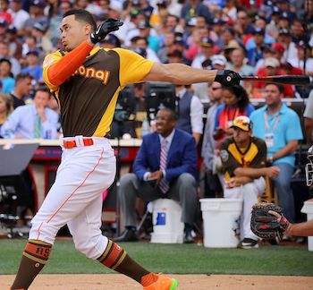
This is Giancarlo Stanton. He is also a very large human being, standing 6 feet 6 inches tall and weighing 245 pounds. Despite not wearing the same jersey as Judge in the pictures provided, in 2018 they will be teammates on the New York Yankees. They are similar in a lot of ways, one being that they hit a lot of home runs. Stanton and Judge led baseball in home runs in 2017, with 59 and 52, respectively. These are exceptional totals - the player in third “only” had 45 home runs.

Stanton and Judge are also different in many ways. One is batted ball events, which is any batted ball that produces a result. This includes outs, hits, and errors. Next, you’ll find the counts of batted ball events for each player in 2017. The frequencies of other events are quite different.

# All of Aaron Judge's batted ball events in 2017
judge_events_2017 = judge.loc[judge.game_year == 2017,:]['events']
print("Aaron Judge batted ball event totals, 2017:")
print(judge_events_2017.value_counts())

Aaron Judge batted ball event totals, 2017: strikeout 207 field_out 146 walk 116 single 75 home_run 52 double 24 grounded_into_double_play 15 intent_walk 11 force_out 11 hit_by_pitch 5 sac_fly 4 field_error 4 fielders_choice_out 4 triple 3 strikeout_double_play 1 Name: events, dtype: int64

# All of Giancarlo Stanton's batted ball events in 2017
stanton_events_2017 = stanton.loc[stanton.game_year == 2017,:]['events']
print("\nGiancarlo Stanton batted ball event totals, 2017:")
print(stanton_events_2017.value_counts())

Giancarlo Stanton batted ball event totals, 2017: field_out 239 strikeout 161 single 77 walk 72 home_run 59 double 32 intent_walk 13 grounded_into_double_play 13 hit_by_pitch 7 force_out 7 field_error 5 sac_fly 3 strikeout_double_play 2 fielders_choice_out 2 pickoff_1b 1 Name: events, dtype: int64

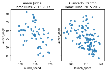
18.1.4 Analyzing home runs with Statcast data

So Judge walks and strikes out more than Stanton. Stanton flies out more than Judge. But let’s get into their hitting profiles in more detail. Two of the most groundbreaking Statcast metrics are launch angle and exit velocity:

Launch angle: the vertical angle at which the ball leaves a player’s bat
Exit velocity: the speed of the baseball as it comes off the bat

This new data has changed the way teams value both hitters and pitchers. Why? As per the Washington Post:

Balls hit with a high launch angle are more likely to result in a hit. Hit fast enough and at the right angle, they become home runs.

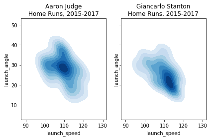
Let’s look at exit velocity vs. launch angle and let’s focus on home runs only (2015-2017). The first two plots show data points. The second two show smoothed contours to represent density.

judge.columns.values

array([‘pitch_type’, ‘game_date’, ‘release_speed’, ‘release_pos_x’, ‘release_pos_z’, ‘player_name’, ‘batter’, ‘pitcher’, ‘events’, ‘description’, ‘spin_dir’, ‘spin_rate_deprecated’, ‘break_angle_deprecated’, ‘break_length_deprecated’, ‘zone’, ‘des’, ‘game_type’, ‘stand’, ‘p_throws’, ‘home_team’, ‘away_team’, ‘type’, ‘hit_location’, ‘bb_type’, ‘balls’, ‘strikes’, ‘game_year’, ‘pfx_x’, ‘pfx_z’, ‘plate_x’, ‘plate_z’, ‘on_3b’, ‘on_2b’, ‘on_1b’, ‘outs_when_up’, ‘inning’, ‘inning_topbot’, ‘hc_x’, ‘hc_y’, ‘tfs_deprecated’, ‘tfs_zulu_deprecated’, ‘pos2_person_id’, ‘umpire’, ‘sv_id’, ‘vx0’, ‘vy0’, ‘vz0’, ‘ax’, ‘ay’, ‘az’, ‘sz_top’, ‘sz_bot’, ‘hit_distance_sc’, ‘launch_speed’, ‘launch_angle’, ‘effective_speed’, ‘release_spin_rate’, ‘release_extension’, ‘game_pk’, ‘pos1_person_id’, ‘pos2_person_id.1’, ‘pos3_person_id’, ‘pos4_person_id’, ‘pos5_person_id’, ‘pos6_person_id’, ‘pos7_person_id’, ‘pos8_person_id’, ‘pos9_person_id’, ‘release_pos_y’, ‘estimated_ba_using_speedangle’, ‘estimated_woba_using_speedangle’, ‘woba_value’, ‘woba_denom’, ‘babip_value’, ‘iso_value’, ‘launch_speed_angle’, ‘at_bat_number’, ‘pitch_number’], dtype=object)

# Filter to include home runs only
judge_hr = judge[judge.events == 'home_run']
stanton_hr = stanton[stanton.events == 'home_run']

# Create a figure with two scatter plots of launch speed vs. launch angle, one for each player's home runs
fig1, axs1 = plt.subplots(ncols=2, sharex=True, sharey=True)
sns.regplot(x='launch_speed', y='launch_angle', fit_reg=False, color='tab:blue', data=judge_hr, ax=axs1[0]).set_title('Aaron Judge\nHome Runs, 2015-2017')
sns.regplot(x='launch_speed', y='launch_angle', fit_reg=False, color='tab:blue', data=stanton_hr, ax=axs1[1]).set_title('Giancarlo Stanton\nHome Runs, 2015-2017')

# Create a figure with two KDE plots of launch speed vs. launch angle, one for each player's home runs
fig2, axs2 = plt.subplots(ncols=2, sharex=True, sharey=True)
sns.kdeplot(judge_hr.launch_speed, judge_hr.launch_angle, cmap="Blues", shade=True, shade_lowest=False, ax=axs2[0]).set_title('Aaron Judge\nHome Runs, 2015-2017')
sns.kdeplot(stanton_hr.launch_speed, stanton_hr.launch_angle, cmap="Blues", shade=True, shade_lowest=False, ax=axs2[1]).set_title('Giancarlo Stanton\nHome Runs, 2015-2017')

Text(0.5,1,‘Giancarlo StantonRuns, 2015-2017’)

png

18.1.5 Home runs by pitch velocity

It appears that Stanton hits his home runs slightly lower and slightly harder than Judge, though this needs to be taken with a grain of salt given the small sample size of home runs.

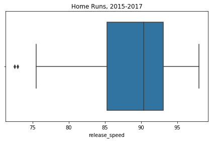
Not only does Statcast measure the velocity of the ball coming off of the bat, it measures the velocity of the ball coming out of the pitcher’s hand and begins its journey towards the plate. We can use this data to compare Stanton and Judge’s home runs in terms of pitch velocity. Next you’ll find box plots displaying the five-number summaries for each player: minimum, first quartile, median, third quartile, and maximum.

# Combine the Judge and Stanton home run DataFrames for easy boxplot plotting
judge_stanton_hr = pd.concat([judge_hr,stanton_hr])

# Create a boxplot that describes the pitch velocity of each player's home runs
sns.boxplot(judge_stanton_hr['release_speed'], color = 'tab:blue').set_title('Home Runs, 2015-2017')

Text(0.5,1,‘Home Runs, 2015-2017’)

png

18.1.6 Home runs by pitch location (I)

So Judge appears to hit his home runs off of faster pitches than Stanton. We might call Judge a fastball hitter. Stanton appears agnostic to pitch speed and likely pitch movement since slower pitches (e.g. curveballs, sliders, and changeups) tend to have more break. Statcast does track pitch movement and type but let’s move on to something else: pitch location. Statcast tracks the zone the pitch is in when it crosses the plate. The zone numbering looks like this (from the catcher’s point of view):

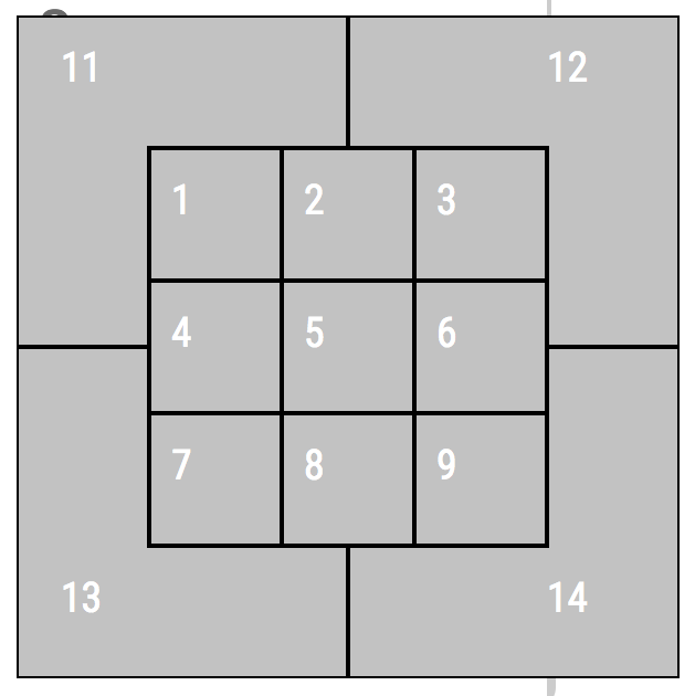
We can plot this using a 2D histogram. For simplicity, let’s only look at strikes, which gives us a 9x9 grid. We can view each zone as coordinates on a 2D plot, the bottom left corner being (1,1) and the top right corner being (3,3). Let’s set up a function to assign x-coordinates to each pitch.

def assign_x_coord(row):
    """
    Assigns an x-coordinate to Statcast's strike zone numbers. Zones 11, 12, 13,
    and 14 are ignored for plotting simplicity.
    """
    # Left third of strike zone
    if row.zone in [1, 4, 7]:
        return 1
    # Middle third of strike zone
    if row.zone in [2, 5, 8]:
        return 2
    # Right third of strike zone
    if row.zone in [3, 6, 9]:
        return 3

18.1.7 Home runs by pitch location (II)

And let’s do the same but for y-coordinates.

def assign_y_coord(row):
    """
    Assigns a y-coordinate to Statcast's strike zone numbers. Zones 11, 12, 13,
    and 14 are ignored for plotting simplicity.
    """
    # Upper third of strike zone
    if row.zone in [1,2,3]:
        return 3
    # Middle third of strike zone
    if row.zone in [4,5,6]:
        return 2
    # Lower third of strike zone
    if row.zone in [7,8,9]:
        return 1

18.1.8 Aaron Judge’s home run zone

Now we can apply the functions we’ve created then construct our 2D histograms. First, for Aaron Judge (again, for pitches in the strike zone that resulted in home runs).

# Zones 11, 12, 13, and 14 are to be ignored for plotting simplicity
judge_strike_hr = judge_hr.copy().loc[judge_hr.zone <= 9]

# Assign Cartesian coordinates to pitches in the strike zone for Judge home runs
judge_strike_hr['zone_x'] = judge_strike_hr.apply(assign_x_coord, axis = 1)
judge_strike_hr['zone_y'] = judge_strike_hr.apply(assign_y_coord, axis = 1)

# Plot Judge's home run zone as a 2D histogram with a colorbar
plt.hist2d(judge_strike_hr['zone_x'], judge_strike_hr['zone_y'], bins = 3, cmap='Blues')
plt.title('Aaron Judge Home Runs on\n Pitches in the Strike Zone, 2015-2017')
plt.gca().get_xaxis().set_visible(False)
plt.gca().get_yaxis().set_visible(False)
cb = plt.colorbar()
cb.set_label('Counts in Bin')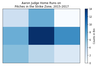

png

18.1.9 Giancarlo Stanton’s home run zone

And now for Giancarlo Stanton.

# Zones 11, 12, 13, and 14 are to be ignored for plotting simplicity
stanton_strike_hr = stanton_hr.copy().loc[stanton_hr.zone <= 9]

# Assign Cartesian coordinates to pitches in the strike zone for Stanton home runs
stanton_strike_hr['zone_x'] = stanton_strike_hr.apply(assign_x_coord, axis=1)
stanton_strike_hr['zone_y'] = stanton_strike_hr.apply(assign_y_coord, axis=1)

# Plot Stanton's home run zone as a 2D histogram with a colorbar
plt.hist2d(stanton_strike_hr['zone_x'], stanton_strike_hr['zone_y'], bins = 3, cmap='Blues')
plt.title('Giancarlo Stanton Home Runs on\n Pitches in the Strike Zone, 2015-2017')
plt.gca().get_xaxis().set_visible(False)
plt.gca().get_yaxis().set_visible(False)
cb = plt.colorbar()
cb.set_label('Counts in Bin')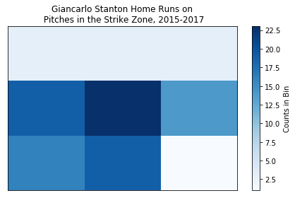

png

18.1.10 Should opposing pitchers be scared?

A few takeaways:

Stanton does not hit many home runs on pitches in the upper third of the strike zone.
Like pretty much every hitter ever, both players love pitches in the horizontal and vertical middle of the plate.
Judge’s least favorite home run pitch appears to be high-away while Stanton’s appears to be low-away.
If we were to describe Stanton’s home run zone, it’d be middle-inside. Judge’s home run zone is much more spread out.

The grand takeaway from this whole exercise: Aaron Judge and Giancarlo Stanton are not identical despite their superficial similarities. In terms of home runs, their launch profiles, as well as their pitch speed and location preferences, are different.

Should opposing pitchers still be scared?

# Should opposing pitchers be wary of Aaron Judge and Giancarlo Stanton
should_pitchers_be_scared = ...

参考文献

Datawhale. 2020. “50道练习实践学习Pandas！.” Datawhale. 2020. https://mp.weixin.qq.com/s/XmnWvnMNobuF-92vbppNbQ.

Friedman, Howard. 2020. “Which Debts Are Worth the Bank’s Effort?” DataCamp. 2020. https://www.datacamp.com/projects/504.

Leung, Deo. 2018. “How Floor a Date to the First Date of That Month?” Stack Overflow. 2018. https://stackoverflow.com/a/49869631/8625228.

Orac, Roman. 2020. “不容错过的Pandas小技巧：万能转格式、轻松合并、压缩数据，让数据分析更高效.” 量子位. 2020. https://mp.weixin.qq.com/s/RY9efkvdPE5JJq6UWWOFFw.

Reback, Jeff. 2017. “Can’t Use Dt.ceil, Dt.floor, Dt.round with Coarser Target Frequencies.” GitHub. 2017. https://github.com/pandas-dev/pandas/issues/15303#issuecomment-277401817.

Venturi, David. 2020. “A New Era of Data Analysis in Baseball.” DataCamp. 2020. https://www.datacamp.com/projects/250.

易执. 2020. “Pandas数据分析——超好用的Groupby详解.” Python读数. 2020. https://mp.weixin.qq.com/s/9OoNH8MMpYlZhABGjGvvzQ.

Pandas Cookbook

Pandas Cookbook

1 floor 到每周处理方法

2 groupby

3 pandas 1.0.0

4 import pandas series

5 cut number

6 plot

7 groupby 看统计结果

8 插入新行

9 loc 用数字 index

10 pandas 保存 zip

11 文本直接相加

12 `pd.to_datetime` 用 apply

13 指定列 fillna

14 groupby 怎么拿到 index

15 reshape 1D to df

16 pull value from pandas df

17 subset series by multiple index

18 to_csv OSError

附录

18.1 棒球数据案例

18.1.1 The Statcast revolution

18.1.2 What can Statcast measure?

18.1.3 Aaron Judge and Giancarlo Stanton, prolific sluggers

18.1.4 Analyzing home runs with Statcast data

18.1.5 Home runs by pitch velocity

18.1.6 Home runs by pitch location (I)

18.1.7 Home runs by pitch location (II)

18.1.8 Aaron Judge’s home run zone

18.1.9 Giancarlo Stanton’s home run zone

18.1.10 Should opposing pitchers be scared?

参考文献

	company	salary	age
0	A	19	17
1	A	39	42
2	A	29	19
3	C	20	46
4	C	41	16
5	A	48	28
6	C	21	34
7	B	14	19
8	C	34	42
9	C	27	18

	company	salary	age
0	A	19	17
1	A	39	42
2	A	29	19
3	C	20	46
4	C	41	16
5	A	48	28
6	C	21	34
7	B	14	19
8	C	34	42
9	C	27	18

Pandas Cookbook

1 floor 到每周处理方法

2 groupby

3 pandas 1.0.0

4 import pandas series

5 cut number

6 plot

7 groupby 看统计结果

8 插入新行

9 loc 用数字 index

10 pandas 保存 zip

11 文本直接相加

12 pd.to_datetime 用 apply

13 指定列 fillna

14 groupby 怎么拿到 index

15 reshape 1D to df

16 pull value from pandas df

17 subset series by multiple index

18 to_csv OSError

附录

18.1 棒球数据案例

18.1.1 The Statcast revolution

18.1.2 What can Statcast measure?

18.1.3 Aaron Judge and Giancarlo Stanton, prolific sluggers

18.1.4 Analyzing home runs with Statcast data

18.1.5 Home runs by pitch velocity

18.1.6 Home runs by pitch location (I)

18.1.7 Home runs by pitch location (II)

18.1.8 Aaron Judge’s home run zone

18.1.9 Giancarlo Stanton’s home run zone

18.1.10 Should opposing pitchers be scared?

参考文献

12 `pd.to_datetime` 用 apply

	company	salary	age
0	A	19	17
1	A	39	42
2	A	29	19
3	C	20	46
4	C	41	16
5	A	48	28
6	C	21	34
7	B	14	19
8	C	34	42
9	C	27	18