learn_pul

A Minimal Example of PU Learning Using R

李家翔 2019-02-26

数据来自

from sklearn.datasets.samples_generator import make_blobs

以下实验的目的是检验当部分正样本和全部负样本未知的情况下，比较PU Learning 的模型效果和 已经全部正负样本下的模型结果。

如果两个结果差异不大，表示 PU Learning 明显效果不错。

suppressMessages(library(tidyverse))
x <- read_csv("datasets/make_circles_x.csv")

## Parsed with column specification:
## cols(
##   feature1 = col_double(),
##   feature2 = col_double()
## )

y <- read_csv("datasets/make_circles_y.csv")

## Parsed with column specification:
## cols(
##   y = col_double()
## )

table(y)

## y
##    0    1 
## 3000 3000

head(x)

## # A tibble: 6 x 2
##   feature1 feature2
##      <dbl>    <dbl>
## 1    0.789     3.79
## 2    6.66      5.88
## 3    0.440    -1.47
## 4    0.334     4.32
## 5    4.92      4.28
## 6    5.82      2.74

假设 2700 个正样本是未知的，所有的负样本是未知的。

set.seed(123)
unlabelled_index <- sample(x = which(y == 1),size = 2700,replace = F)
y_new <- y
y_new[unlabelled_index,]$y <- 0

data <- bind_cols(y_new,x)
table(data$y)

## 
##    0    1 
## 5700  300

table(y)

## y
##    0    1 
## 3000 3000

library(randomForest)

## randomForest 4.6-14

## Type rfNews() to see new features/changes/bug fixes.

## 
## Attaching package: 'randomForest'

## The following object is masked from 'package:dplyr':
## 
##     combine

## The following object is masked from 'package:ggplot2':
## 
##     margin

model <- randomForest(as.factor(y) ~ feature1 + feature2, data = data)

yhat <- predict(model,type = 'prob')[,2]

ks_table <- function(yhat, y) {
  library(tidyverse)
  pred <- ROCR::prediction(yhat, y)
  perf <- ROCR::performance(pred, 'tpr', 'fpr') 
  # tpr true positive rate
  # fpr false positive rate
  perf_df <- data.frame(perf@x.values, perf@y.values) 
  names(perf_df) <- c("fpr", "tpr")
  per_df2 <- 
    perf_df %>% 
    mutate(cutoff = 1:nrow(.)/nrow(.)) %>% 
    mutate(ks = tpr - fpr)
  return(per_df2)
}

ks_table(yhat,y) %>% 
    gather(key,value, tpr,fpr,ks) %>% 
    ggplot(aes(x = cutoff, y = value, col = key)) +
    geom_line()

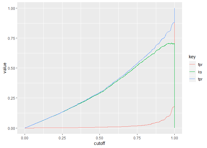
看到 KS 可以达到 70% 左右，因此模型效果并不差。

那么假设正样本和负样本完全已知的情况下，对比简单模型效果。

data2 <- bind_cols(y,x)
model2 <- randomForest(as.factor(y) ~ feature1 + feature2, data = data2)

yhat2 <- predict(model2,type = 'prob')[,2]

ks_table(yhat2,y) %>% 
    gather(key,value, tpr,fpr,ks) %>% 
    ggplot(aes(x = cutoff, y = value, col = key)) +
    geom_line()

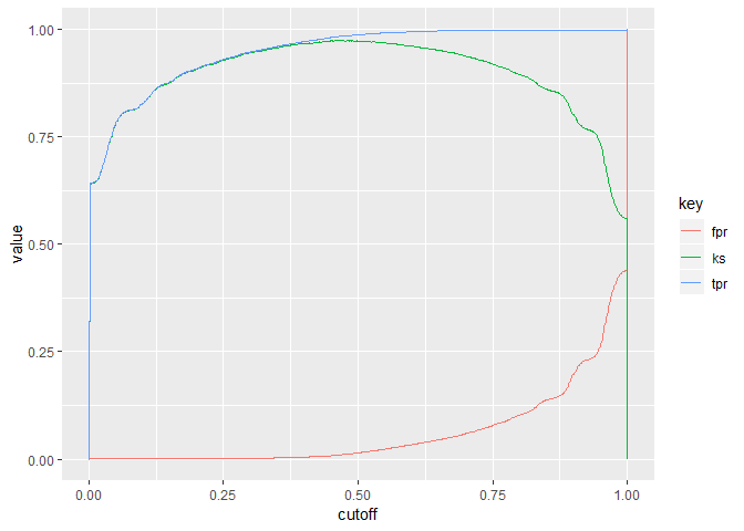
KS 为 100%，这是因为 feature1 和 feature2 本身是完全有效的两个变量。 对比前者 KS 差异 1/3 的准确性，因此是可以接受的。

PU Learning 的结果并不差。