使用 RMarkdown 的 child 参数，进行文档拼接。
这样拼接以后的笔记方便复习。
相关问题提交到 Issue

Souliotis (2019) 主要讲解了 grouped 的运算、替代函数、向量化内容。相关实现代码见各个章节 labs 小节。

1 subset df

1.1 efficient code

Why we need efficient code and how to measure it (Souliotis 2019)

高效代码的定义，保证相同逻辑下执行快。

1.2 基本统计运算

The NumPy function is faster in calculating basic statistical functions on pandas series. (Souliotis 2019)

基本统计运算 numpy 是快于 pandas

pd_start_time = time.time()

# Calculate the variance using pandas
print(poker_hands['R2'].var())

# Print the CPU time required to complete the operation 
print("Results from the pandas method calculated in %s seconds" % (time.time() - pd_start_time))

np_start_time = time.time()

# Calculate the variance using NumPy
print(np.var(poker_hands['R2']))

# Print the CPU time required to complete the operation 
print("Results from the NumPy method calculated in %s seconds" % (time.time() - np_start_time))

1.3 Locate rows

image

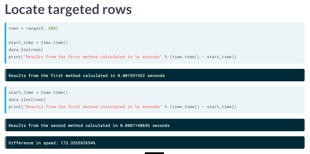
iloc 会更快。

image

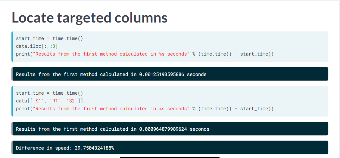
但是指定 column 时， loc 更快。

iloc() is faster for selecting specific rows. (Souliotis 2019) loc() is faster works better for selecting columns. (Souliotis 2019)

# Define the variable that keeps the targeted indices
rows = range(0,1000)

# Select the rows using the targeted indices and calculate the CPU time
loc_start_time = time.time()
print(poker_hands.loc[rows].head())
print("Results from the .loc method calculated in %s seconds" % (time.time() - loc_start_time))

#Select the rows using the targeted indices and calculate the CPU time
iloc_start_time = time.time()
print(poker_hands.iloc[rows].head())
print("Results from the .iloc method calculated in %s seconds" % (time.time() - iloc_start_time))

.iloc() takes advantages of the sorted position of each rows, simplifying the computations needed. (Souliotis 2019)

# Use .iloc to select the first 6 columns 
ind_start_time = time.time()
print(poker_hands.iloc[:,0:6])
print("Results from the first method calculated in %s seconds" % (time.time() - ind_start_time))

# Use simple column selection to select the first 6 columns 
name_start_time = time.time()
print(poker_hands[['S1', 'R1', 'S2', 'R2', 'S3', 'R3']])
print("Results from the second method calculated in %s seconds" % (time.time() - name_start_time))

1.4 Select random rows

# Extract number of rows in dataset
N=poker_hands.shape[0]

# Select and time the selection of the 75% of the dataset's rows
rand_start_time = time.time()
poker_hands.iloc[np.random.randint(low=0, high=N, size=int(0.75 * N))]
print("Results from the first method calculated in %s seconds" % (time.time() - rand_start_time))

# Select and time the selection of the 75% of the dataset's rows using sample()
samp_start_time = time.time()
poker_hands.sample(int(0.75 * N), axis=0, replace = True)
print("Results from the second method calculated in %s seconds" % (time.time() - samp_start_time))

pandas 比 numpy 快。

# Extract number of columns in dataset
D=poker_hands.shape[1]

# Select and time the selection of 4 of the dataset's columns using NumPy
np_start_time = time.time()
poker_hands.iloc[:,np.random.randint(low=0, high=D, size=4)]
print("Results from the first method calculated in %s seconds" % (time.time() - np_start_time))

# Select and time the selection of 4 of the dataset's columns using pandas
pd_start_time = time.time()
poker_hands.sample(4, axis=1)
print("Results from the second method calculated in %s seconds" % (time.time() - pd_start_time))

column 也是 pandas 快。

1.5 lab 1

1.6 lab 2

2 replace

2.1 .replace()

比直接赋值要快很多，且代码简洁。

start_time = time.time()

# Replace all the entries that has 'FEMALE' as a gender with 'GIRL'
names['Gender'][names['Gender']=='FEMALE'] = 'GIRL'

print("Results from the first method calculated in %s seconds" % (time.time() - start_time))

start_time = time.time()

# Replace all the entries that has 'FEMALE' as a gender with 'GIRL'
names['Gender'].replace('FEMALE', 'GIRL', inplace=True)

print("Results from the first method calculated in %s seconds" % (time.time() - start_time))

start_time = time.time()

# Replace all non-Hispanic ethnicities with 'NON HISPANIC'
names['Ethnicity'].loc[(names["Ethnicity"] == 'BLACK NON HISPANIC') | 
                      (names["Ethnicity"] == 'BLACK NON HISP') | 
                      (names["Ethnicity"] == 'WHITE NON HISPANIC') | 
                      (names["Ethnicity"] == 'WHITE NON HISP')] = 'NON HISPANIC'

print("Results from the above operation calculated in %s seconds" % (time.time() - start_time))

start_time = time.time()

# Replace all non-Hispanic ethnicities with 'NON HISPANIC'
names['Ethnicity'].replace(['BLACK NON HISP', 'BLACK NON HISPANIC', 'WHITE NON HISP' , 'WHITE NON HISPANIC'], ['NON HISPANIC','NON HISPANIC','NON HISPANIC','NON HISPANIC'], inplace=True)

print("Results from the above operation calculated in %s seconds" % (time.time() - start_time))

In general, working with dictionaries in Python is very efficient compared to lists looking through a list requires. (Souliotis 2019) Looking through a list requires a pass in every element of the list, while looking at a dictionary directs instantly to the key that matches the entry. (Souliotis 2019)

因此不同情况使用时，

list 是单个情况，用 list，因为方便，减少开发时间 dict 是多个情况，用 dict，因为方便，减少开发时间，且跑得快。

Replace every rowof the DataFrame listed as ‘Royal flush’ or ‘Straight flush’ in the ‘Explanation’ column to ‘Flush’. (Souliotis 2019)

# Replace Royal flush or Straight flush to Flush
poker_hands.replace({'Royal flush':'Flush', 'Straight flush':'Flush'}, inplace=True)
print(poker_hands['Explanation'].head())

2.2 自动改变变量类型

# Replace the number rank by a string
names['Rank'].replace({1:'FIRST', 2:'SECOND', 3:'THIRD'}, inplace=True)
print(names.head())

In [2]: names.info()
<class 'pandas.core.frame.DataFrame'>
RangeIndex: 11345 entries, 0 to 11344
Data columns (total 6 columns):
Year of Birth         11345 non-null int64
Gender                11345 non-null object
Ethnicity             11345 non-null object
Child's First Name    11345 non-null object
Count                 11345 non-null int64
Rank                  11345 non-null int64
dtypes: int64(3), object(3)
memory usage: 531.9+ KB

Rank 11345 non-null int64 是 int

    <class 'pandas.core.frame.DataFrame'>
    RangeIndex: 11345 entries, 0 to 11344
    Data columns (total 6 columns):
    Year of Birth         11345 non-null int64
    Gender                11345 non-null object
    Ethnicity             11345 non-null object
    Child's First Name    11345 non-null object
    Count                 11345 non-null int64
    Rank                  11345 non-null object
    dtypes: int64(2), object(4)
    memory usage: 531.9+ KB

As you saw in the video, you can use dictionaries to replace multiple values with just one value, even from multiple columns. (Souliotis 2019)

# Replace the rank of the first three ranked names to 'MEDAL'
names.replace({'Rank': {1:'MEDAL', 2:'MEDAL', 3:'MEDAL'}}, inplace=True)

# Replace the rank of the 4th and 5th ranked names to 'ALMOST MEDAL'
names.replace({'Rank': {4:'ALMOST MEDAL', 5:'ALMOST MEDAL'}}, inplace=True)
print(names.head())

2.3 labs

3 向量化

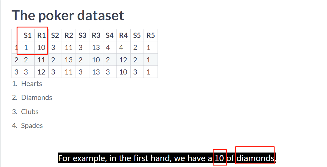
3.1 数据集介绍

image

两个标签，一个是花色，一个是数字。每行是一手，一手有五张。

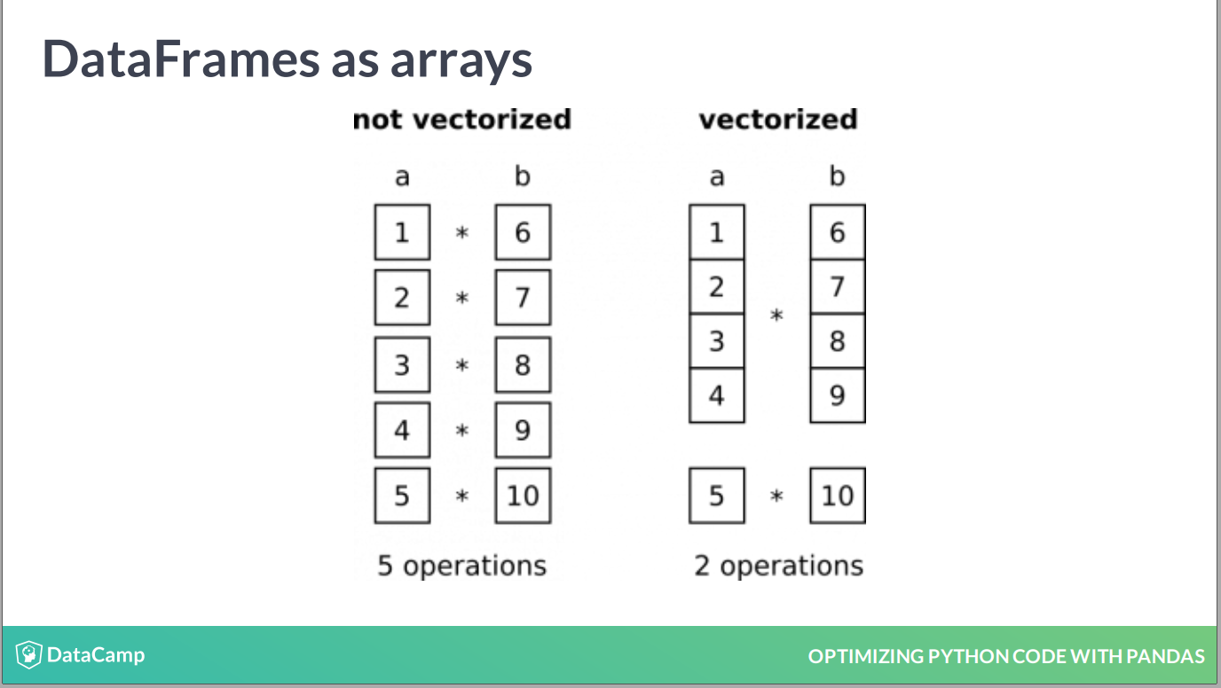
3.2 向量化

vectorization is the most efficient way to achieve it. (Souliotis 2019) (Souliotis 2019)

image

向量化指对类似的数据类型，进行同样的运算法则，类似于 SQL中的 partition。

3.3 .iterrows

.iterrows() 就是把 df 变成 generator，一行是一个对象。

It is very similar to the notation of the enumerate() function, (Souliotis 2019) which when applied to a list returns each element along with its index. (Souliotis 2019)

这个可以在 lab 里面查看到。但是.iterrows()很慢！但是是一个更加清晰的方式，让我们理解迭代。

我怎么就继续学习了，没有好好用 jupyter notebook 去总结呢？

Each time you iterate through it, it will yield two elements: (Souliotis 2019)

the index of the respective row (Souliotis 2019)

a pandas Series with all the elements of that row (Souliotis 2019) Then, you will print all the elements of the 2nd row, using the generator. (Souliotis 2019)

# Create a generator over the rows
generator = poker_hands.iterrows()

# Access the elements of the 2nd row
first_element = next(generator)
second_element = next(generator)
print(first_element, second_element)

<script.py> output:
    (0, S1        1
    R1       10
    S2        1
    R2       11
    S3        1
    R3       13
    S4        1
    R4       12
    S5        1
    R5        1
    Class     9
    Name: 0, dtype: int64) (1, S1        2
    R1       11
    S2        2
    R2       13
    S3        2
    R3       10
    S4        2
    R4       12
    S5        2
    R5        1
    Class     9
    Name: 1, dtype: int64)

反馈的是一个 tuple 格式，可以用 a, b in tuple 解析。

data_generator = poker_hands.iterrows()

for index, values in data_generator:
    # Check if index is odd
    if (index+1) % 2 == 0:
        # Sum the ranks of all the cards
        hand_sum = sum([values[1], values[3], values[5], values[7], values[9]])

3.4 .apply

.apply(lambda x: , axis = 1)

# Define the lambda transformation
get_square = lambda x: np.sqrt(x)

# Apply the transformation
data_sum = poker_hands.apply(get_square)
print(data_sum.head())

3.5 Vectorization over pandas series

recall that the fundamental unit5 of Pandas, DataFrames and Series, are both based on arrays. (Souliotis 2019)

都是 numpy 的结构。

Vectorization is the process of executing operations on entire arrays (Souliotis 2019)

而不是一个个对象进行处理。

# Calculate the mean rank in each hand
start_time = time.time()
mean_r = poker_hands[['R1', 'R2', 'R3', 'R4', 'R5']].mean(axis=1)
print("Results from the above operation calculated in %s seconds" % (time.time() - start_time))
print(mean_r.head())

# Calculate the mean rank of each of the 5 card in all hands
start_time = time.time()
mean_c = poker_hands[['R1', 'R2', 'R3', 'R4', 'R5']].mean(axis=0)
print("Results from the above operation calculated in %s seconds" % (time.time() - start_time))
print(mean_c.head())

默认情况下 python 都是对 column 进行运算，因此 axis = 0 作为默认，是得到每列的汇总值。

3.6 Vectorization with NumPy arrays using .values()

leave out many operations such as indexing, data type checking, etc. (Souliotis 2019) As a result, operations on NumPy arrays can be significantly faster than operations on pandas Series.

ndarrays 比 series 的区别也就是更加简单。这是跑得快的证明(可以见 labs)。

# Calculate the variance in each hand
start_time = time.time()
poker_var = poker_hands[["R1", "R2", "R3", "R4", "R5"]].var(axis=1)
print("Results from the above operation calculated in %s seconds" % (time.time() - start_time))
print(poker_var.head())

# Calculate the variance in each hand
start_time = time.time()
poker_var = poker_hands[["R1", "R2", "R3", "R4", "R5"]].values.var(axis=1, ddof=1)
print("Results from the above operation calculated in %s seconds" % (time.time() - start_time))
print(poker_var[0:5])

<script.py> output:
    Results from the above operation calculated in 0.011882305145263672 seconds
    0    23.3
    1    23.3
    2    23.3
    3    23.3
    4    23.3
    dtype: float64

<script.py> output:
    Results from the above operation calculated in 0.005125284194946289 seconds
    [23.3 23.3 23.3 23.3 23.3]

3.7 labs

4 groups

applying functions on groups of entries. (Souliotis 2019)

处理 groups。

4.1 transoform 和 apply 的区别

The .transform() function applies a function to all members of each group. (Souliotis 2019)

这算是一个特征。

参考 https://stackoverflow.com/a/27951930/8625228 和 https://stackoverflow.com/a/13854901/8625228 针对 group 对象时，apply 只能针对于一个 pd.Series 进行完成，因此对象应该是 pd.DataFrame.groupby().[].apply()，但是 transform 可以针对 group 对象里面的每一列，如 pd.DataFrame.groupby().transfrom(func) 时，实际上是执行

pd.DataFrame.groupby().['col1'].transfrom(func)
pd.DataFrame.groupby().['col2'].transfrom(func)
pd.DataFrame.groupby().['col3'].transfrom(func)
…

library(reticulate)

import pandas as pd
df = r.mtcars
df.head()

##                     mpg  cyl   disp     hp  drat  ...   qsec   vs   am  gear  carb
## Mazda RX4          21.0  6.0  160.0  110.0  3.90  ...  16.46  0.0  1.0   4.0   4.0
## Mazda RX4 Wag      21.0  6.0  160.0  110.0  3.90  ...  17.02  0.0  1.0   4.0   4.0
## Datsun 710         22.8  4.0  108.0   93.0  3.85  ...  18.61  1.0  1.0   4.0   1.0
## Hornet 4 Drive     21.4  6.0  258.0  110.0  3.08  ...  19.44  1.0  0.0   3.0   1.0
## Hornet Sportabout  18.7  8.0  360.0  175.0  3.15  ...  17.02  0.0  0.0   3.0   2.0
## 
## [5 rows x 11 columns]

df.groupby('cyl')['mpg'].apply(max)

## cyl
## 4.0    33.9
## 6.0    21.4
## 8.0    19.2
## Name: mpg, dtype: float64

df.groupby('cyl')['mpg'].transform(max).head() # 类似于 `mutate(x_min = min(x))`

## Mazda RX4            21.4
## Mazda RX4 Wag        21.4
## Datsun 710           33.9
## Hornet 4 Drive       21.4
## Hornet Sportabout    19.2
## Name: mpg, dtype: float64

4.2 .groupby().transform

# Define the min-max transformation
min_max_tr = lambda x: (x - x.min()) / (x.max() - x.min())

# Group the data according to the time
restaurant_grouped = restaurant_data.groupby('time')

# Apply the transformation
restaurant_min_max_group = restaurant_grouped.transform(min_max_tr)
print(restaurant_min_max_group.head())

这里不用 apply，因为这里的对象是 pd.DataFrame，而不是 pd.Series。

The transformation will be an exponential transformation. The exponential distribution is defined as (Souliotis 2019) \(e^{-\lambda * x} * \lambda\) where \(\lambda\) is the mean of the group that the observation x belongs to. You’re going to apply the exponential distribution transformation to the size of each table in the dataset, after grouping the data according to the time of the day the meal took place. Remember to use each group’s mean for the value of \(\lambda\). (Souliotis 2019)

注意指数分布受制于当前数据集的局部均值。

# Define the exponential transformation
pois_tr = lambda x: np.exp(-x.mean()*x) * x.mean()

# Group the data according to the time
restaurant_grouped = restaurant_data.groupby("time")

# Apply the transformation
restaurant_pois_group = restaurant_grouped['tip'].transform(pois_tr)
print(restaurant_pois_group.head())

zscore = lambda x: (x - x.mean()) / x.std()

# Apply the transformation
poker_trans = poker_grouped.transform(zscore)

# Re-group the grouped object and print each group's means and standard deviation
poker_regrouped = poker_trans.groupby(poker_hands['Class'])

print(np.round(poker_regrouped.mean(), 3))
print(poker_regrouped.std())

<script.py> output:
            S1   R1   S2   R2   S3   R3   S4   R4   S5   R5
    Class                                                  
    0     -0.0 -0.0  0.0 -0.0  0.0  0.0  0.0  0.0 -0.0  0.0
    1      0.0  0.0 -0.0  0.0 -0.0  0.0  0.0  0.0 -0.0  0.0
    2     -0.0 -0.0  0.0 -0.0 -0.0  0.0  0.0 -0.0 -0.0  0.0
    3      0.0  0.0  0.0 -0.0 -0.0 -0.0 -0.0 -0.0  0.0 -0.0
    4     -0.0 -0.0 -0.0 -0.0  0.0 -0.0 -0.0  0.0  0.0  0.0
    5     -0.0 -0.0 -0.0  0.0 -0.0  0.0 -0.0 -0.0 -0.0  0.0
    6     -0.0 -0.0 -0.0  0.0  0.0 -0.0  0.0  0.0 -0.0  0.0
    7      0.0 -0.0 -0.0  0.0 -0.0  0.0  0.0 -0.0 -0.0 -0.0
    8     -0.0  0.0 -0.0  0.0 -0.0  0.0 -0.0  0.0 -0.0 -0.0
    9      0.0 -0.0  0.0 -0.0  0.0 -0.0  0.0  0.0  0.0 -0.0
            S1   R1   S2   R2   S3   R3   S4   R4   S5   R5
    Class                                                  
    0      1.0  1.0  1.0  1.0  1.0  1.0  1.0  1.0  1.0  1.0
    1      1.0  1.0  1.0  1.0  1.0  1.0  1.0  1.0  1.0  1.0
    2      1.0  1.0  1.0  1.0  1.0  1.0  1.0  1.0  1.0  1.0
    3      1.0  1.0  1.0  1.0  1.0  1.0  1.0  1.0  1.0  1.0
    4      1.0  1.0  1.0  1.0  1.0  1.0  1.0  1.0  1.0  1.0
    5      1.0  1.0  1.0  1.0  1.0  1.0  1.0  1.0  1.0  1.0
    6      1.0  1.0  1.0  1.0  1.0  1.0  1.0  1.0  1.0  1.0
    7      1.0  1.0  1.0  1.0  1.0  1.0  1.0  1.0  1.0  1.0
    8      1.0  1.0  1.0  1.0  1.0  1.0  1.0  1.0  1.0  1.0
    9      1.0  1.0  1.0  1.0  1.0  1.0  1.0  1.0  1.0  1.0

4.3 缺失值补充


# Define the lambda function
missing_trans = lambda x: x.fillna(x.median())

其实这么看来这是 define 函数一个更加 Python 的写法。

replace missing values in a dataset groupwise! (Souliotis 2019)

# Define the lambda function
missing_trans = lambda x: x.fillna(x.median())

# Group the data according to time
restaurant_grouped = restaurant_data.groupby("time")

# Apply the transformation
restaurant_impute = restaurant_grouped.transform(missing_trans)
print(restaurant_impute.head())

4.4 filter()

subset the dataset in a groupwise (Souliotis 2019)

# Filter the days where the count of total_bill is greater than $40
total_bill_40 = restaurant_data.groupby('day').filter(lambda x: x['total_bill'].count() > 40)

# Print the number of tables where total_bill is greater than $40
print('Number of tables where total_bill is greater than $40:', total_bill_40.shape[0])

这是筛选 grouped df，直接剔除某些组。

# Filter the days where the count of total_bill is greater than $40
total_bill_40 = restaurant_data.groupby('day').filter(lambda x: x['total_bill'].count() > 40)

# Select only the entries that have a mean total_bill greater than $20
total_bill_20 = total_bill_40.groupby('day').filter(lambda x : x['total_bill'].mean() > 20)

# Print days of the week that have a mean total_bill greater than $20
print('Days of the week that have a mean total_bill greater than $20:', total_bill_20.day.unique())

这里的业务逻辑就是去查看有足够量、单价高的周几？

4.5 labs

附录

4.6 函数构建比较

foo = lambda x: f(x)

和

def foo(x):
    f(x)

# Define the lambda transformation
get_variance = lambda x: np.var(x)

# Apply the transformation
data_tr = poker_hands[['R1', 'R2', 'R3', 'R4', 'R5']].apply(get_variance, axis = 1)
print(data_tr.head())

df 就是二维，因此加一个参数作为维度的讨论。

get_variance = lambda x: np.var(x)

# Apply the transformation
data_tr = poker_hands[['R1', 'R2', 'R3', 'R4', 'R5']].apply(get_variance, axis=0)
print(data_tr.head())

4.7 完成证书

参考文献

Souliotis, Leonidas. 2019. “Optimizing Python Code with Pandas.” DataCamp. 2019. https://www.datacamp.com/courses/optimizing-python-code-with-pandas.

Pandas 高效代码学习笔记

Pandas 高效代码学习笔记

1 subset df

1.1 efficient code

1.2 基本统计运算

1.3 Locate rows

1.4 Select random rows

1.5 lab 1

1.6 lab 2

2 replace

2.1 .replace()

2.2 自动改变变量类型

2.3 labs

3 向量化

3.1 数据集介绍

3.2 向量化

3.3 .iterrows

3.4 .apply

3.5 Vectorization over pandas series

3.6 Vectorization with NumPy arrays using .values()

3.7 labs

4 groups

4.1 transoform 和 apply 的区别

4.2 .groupby().transform

4.3 缺失值补充

4.4 filter()

4.5 labs

附录

4.6 函数构建比较

4.7 完成证书

参考文献