使用 RMarkdown 的 child 参数，进行文档拼接。
这样拼接以后的笔记方便复习。
相关问题提交到 Issue

参考 DMLC (2016b)

1 安装¹

install.packages("drat", repos="https://cran.rstudio.com")
drat:::addRepo("dmlc")
install.packages("xgboost", repos="http://dmlc.ml/drat/", type = "source")

2 数据导入

library(xgboost)
library(tidyverse)
data(agaricus.train, package = 'xgboost')
data(agaricus.test, package = 'xgboost')
train <- agaricus.train
test <- agaricus.test

typeof(train)
## [1] "list"
typeof(test)
## [1] "list"
typeof(train$data)
## [1] "S4"
typeof(test$data)
## [1] "S4"

dim(train$data)
## [1] 6513  126
class(train$label)
## [1] "numeric"
dim(test$data)
## [1] 1611  126
class(test$label)
## [1] "numeric"

dgCMatrix which is a sparse² matrix and label vector is a numeric vector ({0,1})

注意这是dgCMatrix数据结构。

dgCMatrix 本身是 sparse matrix 因此不需要使用 r base 函数 sparse matrix 函数，因为对缺失值不友好，不能保留。

str(train)

## List of 2
##  $ data :Formal class 'dgCMatrix' [package "Matrix"] with 6 slots
##   .. ..@ i       : int [1:143286] 2 6 8 11 18 20 21 24 28 32 ...
##   .. ..@ p       : int [1:127] 0 369 372 3306 5845 6489 6513 8380 8384 10991 ...
##   .. ..@ Dim     : int [1:2] 6513 126
##   .. ..@ Dimnames:List of 2
##   .. .. ..$ : NULL
##   .. .. ..$ : chr [1:126] "cap-shape=bell" "cap-shape=conical" "cap-shape=convex" "cap-shape=flat" ...
##   .. ..@ x       : num [1:143286] 1 1 1 1 1 1 1 1 1 1 ...
##   .. ..@ factors : list()
##  $ label: num [1:6513] 1 0 0 1 0 0 0 1 0 0 ...

str(test)

## List of 2
##  $ data :Formal class 'dgCMatrix' [package "Matrix"] with 6 slots
##   .. ..@ i       : int [1:35442] 0 2 7 11 13 16 20 22 27 31 ...
##   .. ..@ p       : int [1:127] 0 83 84 806 1419 1603 1611 2064 2064 2701 ...
##   .. ..@ Dim     : int [1:2] 1611 126
##   .. ..@ Dimnames:List of 2
##   .. .. ..$ : NULL
##   .. .. ..$ : chr [1:126] "cap-shape=bell" "cap-shape=conical" "cap-shape=convex" "cap-shape=flat" ...
##   .. ..@ x       : num [1:35442] 1 1 1 1 1 1 1 1 1 1 ...
##   .. ..@ factors : list()
##  $ label: num [1:1611] 0 1 0 0 0 0 1 0 1 0 ...

2.1 导入方式

bstSparse <- xgboost(data = train$data, 
                     label = train$label, 
                     max.depth = 2, 
                     eta = 1, 
                     nthread = 2, 
                     nround = 2, 
                     objective = "binary:logistic")

## [1]  train-error:0.046522 
## [2]  train-error:0.022263

$\eta$我估计是学习率，$\eta \in [0,1]$。

bstDense <- xgboost(data = as.matrix(train$data), 
                    label = train$label, 
                    max.depth = 2, 
                    eta = 1, 
                    nthread = 2, 
                    nround = 2, 
                    objective = "binary:logistic")

## [1]  train-error:0.046522 
## [2]  train-error:0.022263

dtrain <- xgb.DMatrix(data = train$data, label = train$label)
bstDMatrix <- xgboost(data = dtrain, 
                      max.depth = 2, 
                      eta = 1, 
                      nthread = 2, 
                      nround = 2, 
                      objective = "binary:logistic")

## [1]  train-error:0.046522 
## [2]  train-error:0.022263

xgb.DMatrix将$y$和$x$bind起来。

2.2 xgb.DMatrix

dtrain <- xgb.DMatrix(data = train$data, label = train$label)
dtest <- xgb.DMatrix(data = test$data, label = test$label)

方便使用 watchlist。

watchlist <- list(train = dtrain, testhaha = dtest)

bst <-
    xgb.train(
        data = dtrain,
        max.depth = 2,
        eta = 1,
        nthread = 2,
        nround = 2,
        watchlist = watchlist,
        objective = "binary:logistic"
    )

## [1]  train-error:0.046522    testhaha-error:0.042831 
## [2]  train-error:0.022263    testhaha-error:0.021726

3 配置信息查看 verbose

bst <- xgboost(data = dtrain, max.depth = 2, eta = 1, nthread = 2, nround = 2, objective = "binary:logistic", verbose = 0)
bst
## ##### xgb.Booster
## raw: 1.1 Kb 
## call:
##   xgb.train(params = params, data = dtrain, nrounds = nrounds, 
##     watchlist = watchlist, verbose = verbose, print_every_n = print_every_n, 
##     early_stopping_rounds = early_stopping_rounds, maximize = maximize, 
##     save_period = save_period, save_name = save_name, xgb_model = xgb_model, 
##     callbacks = callbacks, max.depth = 2, eta = 1, nthread = 2, 
##     objective = "binary:logistic")
## params (as set within xgb.train):
##   max_depth = "2", eta = "1", nthread = "2", objective = "binary:logistic", silent = "1"
## xgb.attributes:
##   niter
## callbacks:
##   cb.evaluation.log()
## # of features: 126 
## niter: 2
## nfeatures : 126 
## evaluation_log:
##  iter train_error
##     1    0.046522
##     2    0.022263

bst <- xgboost(data = dtrain, max.depth = 2, eta = 1, nthread = 2, nround = 2, objective = "binary:logistic", verbose = 1)
## [1]  train-error:0.046522 
## [2]  train-error:0.022263
bst
## ##### xgb.Booster
## raw: 1.1 Kb 
## call:
##   xgb.train(params = params, data = dtrain, nrounds = nrounds, 
##     watchlist = watchlist, verbose = verbose, print_every_n = print_every_n, 
##     early_stopping_rounds = early_stopping_rounds, maximize = maximize, 
##     save_period = save_period, save_name = save_name, xgb_model = xgb_model, 
##     callbacks = callbacks, max.depth = 2, eta = 1, nthread = 2, 
##     objective = "binary:logistic")
## params (as set within xgb.train):
##   max_depth = "2", eta = "1", nthread = "2", objective = "binary:logistic", silent = "1"
## xgb.attributes:
##   niter
## callbacks:
##   cb.print.evaluation(period = print_every_n)
##   cb.evaluation.log()
## # of features: 126 
## niter: 2
## nfeatures : 126 
## evaluation_log:
##  iter train_error
##     1    0.046522
##     2    0.022263

bst <- xgboost(data = dtrain, max.depth = 2, eta = 1, nthread = 2, nround = 2, objective = "binary:logistic", verbose = 2)
## [1]  train-error:0.046522 
## [2]  train-error:0.022263
bst
## ##### xgb.Booster
## raw: 1.1 Kb 
## call:
##   xgb.train(params = params, data = dtrain, nrounds = nrounds, 
##     watchlist = watchlist, verbose = verbose, print_every_n = print_every_n, 
##     early_stopping_rounds = early_stopping_rounds, maximize = maximize, 
##     save_period = save_period, save_name = save_name, xgb_model = xgb_model, 
##     callbacks = callbacks, max.depth = 2, eta = 1, nthread = 2, 
##     objective = "binary:logistic")
## params (as set within xgb.train):
##   max_depth = "2", eta = "1", nthread = "2", objective = "binary:logistic", silent = "0"
## xgb.attributes:
##   niter
## callbacks:
##   cb.print.evaluation(period = print_every_n)
##   cb.evaluation.log()
## # of features: 126 
## niter: 2
## nfeatures : 126 
## evaluation_log:
##  iter train_error
##     1    0.046522
##     2    0.022263

verbose = 0, no message
verbose = 1, print evaluation metric
verbose = 2, also print information about tree

4 分类问题

objective = "binary:logistic": we will train a binary classification model ;
max.deph = 2: the trees won’t be deep, because our case is very simple ;
nthread = 2: the number of cpu threads we are going to use;
nround = 2: there will be two passes on the data, the second one will enhance the model by further reducing the difference between ground truth and prediction.

为了SQL翻译方便，建议使用max.deph = 2，不要太深，这样 case when 的嵌套很多。

5 回归问题

bst <- xgb.train(data=dtrain, 
                 booster = "gblinear", 
                 max.depth=2, 
                 nthread = 2, 
                 nround=2, 
                 watchlist=watchlist, 
                 eval.metric = "error", 
                 eval.metric = "logloss", 
                 objective = "binary:logistic")

## [1]  train-error:0.012744    train-logloss:0.192453  testhaha-error:0.014277 testhaha-logloss:0.195995 
## [2]  train-error:0.003071    train-logloss:0.083463  testhaha-error:0.002483 testhaha-logloss:0.085506

reg:linear也可以作为objective的。

In simple cases, it will happen because there is nothing better than a linear algorithm to catch a linear link.

However, decision trees are much better to catch a non linear link between predictors and outcome.

Because there is no silver bullet, we advise you to check both algorithms with your own datasets to have an idea of what to use.

说的很好，线性回归适合抓线性关系，然后决策树适合抓非线性关系。谁更好其实说不清楚。真的很快，比gbm快十倍。

6 预测

pred <- predict(bst, test$data)

# size of the prediction vector
print(length(pred))

## [1] 1611

test$dataone-hot了。

print(head(pred))

## [1] 0.03506050 0.88658363 0.03320464 0.05907830 0.20086876 0.09510834

7 从`xgb.DMatrix`中取出信息

这个矩阵可以取出来信息的，类似于dplyr的select

label = getinfo(dtest, "label")
pred <- predict(bst, dtest)
err <- as.numeric(sum(as.integer(pred > 0.5) != label))/length(label)
print(paste("test-error=", err))

## [1] "test-error= 0.00248292985723153"

8 特征重要性

8.1 理论

在R中，使用xgb.importance和xgb.plot.importance函数 (Chen, He, and Benesty 2018) 导出Importances plot。

DMLC (2016a) 和 Sandhu (2016) 给出了三项指标的解释，

Gain就是信息增益。
Cover表示受到该变量影响的样本比例。
Frequency表示变量使用次数和树的数量的比例。

假设有100个样本，4个变量，3个树。

feature 1在每个树上的用于split时，影响了10，5，2个样本，因此

\[\text{Cover} = 10+5+2 = 17 \to 17/100 = 17 \%\]

feature 1在每个树上的用于split时，分别split了2，1，3次，一共有30次splits，因此

\[\text{Freq} = 2+1+3 = 6 \to 6/30 = 20 \%\]

8.2 计算

参考 Srivastava (2016) 可以提取变量的名称，在importances中体现。

devtools::load_all()
train <- learn_xgboost::train
names <- (train$data@Dimnames)[[2]]
importance_matrix <- xgb.importance(model = bst,feature_names = names)
print(importance_matrix)

##                      Feature  Weight
##   1: spore-print-color=green 2.97886
##   2:     cap-surface=grooves 2.34890
##   3:            odor=pungent 2.20744
##   4:           odor=creosote 2.04349
##   5:       cap-shape=conical 1.95161
##  ---                                
## 122:  stalk-root=rhizomorphs 0.00000
## 123:     veil-type=universal 0.00000
## 124:      ring-type=cobwebby 0.00000
## 125:     ring-type=sheathing 0.00000
## 126:          ring-type=zone 0.00000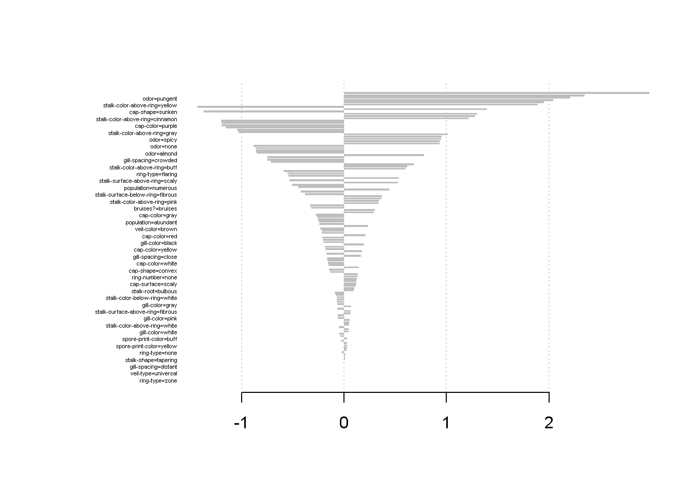

xgb.plot.importance(importance_matrix = importance_matrix)

9 导出树的结构

devtools::load_all()

xgb.dump(bst, with_stats = T)

##   [1] "booster[0]" "bias:"      "-0.0213804" "weight:"    "-1.04406"  
##   [6] "1.95161"    "-0.143276"  "-0.151104"  "0.298288"   "-1.36735"  
##  [11] "-0.509104"  "2.3489"     "0.119476"   "0.338272"   "-0.0701224"
##  [16] "1.01238"    "-0.713659"  "-0.273723"  "-1.19491"   "0.931339"  
##  [21] "-1.19237"   "0.208588"   "-0.15568"   "-0.183115"  "-0.319715" 
##  [26] "0.23697"    "-0.855118"  "-0.855744"  "2.04349"    "0.954912"  
##  [31] "0.782989"   "0.29022"    "-0.882791"  "2.20744"    "0.946141"  
##  [36] "0.125765"   "0"          "0.0276019"  "0"          "0.165364"  
##  [41] "-0.748033"  "0"          "-0.216888"  "0.441682"   "-0.199859" 
##  [46] "-0.170987"  "0.135763"   "0.145828"   "-0.0677529" "1.30117"   
##  [51] "0.023544"   "-0.0585746" "-0.0919774" "-0.164258"  "0.0456166" 
##  [56] "0.0299516"  "-0.0365986" "0.00995269" "0.0951342"  "-0.159782" 
##  [61] "0"          "-0.0443654" "0"          "-0.25558"   "-0.0498434"
##  [66] "0.0656205"  "-0.53132"   "1.28145"    "-0.422857"  "-0.380629" 
##  [71] "-0.543063"  "0.938866"   "-0.260353"  "0.534783"   "0.614559"  
##  [76] "1.21867"    "-1.0265"    "-1.15444"   "0.339209"   "-1.43249"  
##  [81] "0.0508044"  "1.88908"    "0.174663"   "0.371349"   "0.527582"  
##  [86] "-0.864041"  "-0.74868"   "0.195549"   "-1.19887"   "-0.0723885"
##  [91] "1.39598"    "0.0466722"  "0"          "-0.233516"  "-0.205357" 
##  [96] "-0.0657155" "0.601558"   "0.131556"   "0.064248"   "-0.588638" 
## [101] "0"          "0.0515673"  "-0.55054"   "-0.241622"  "-0.0224894"
## [106] "0.0677452"  "0"          "0"          "-0.20858"   "-0.186354" 
## [111] "0.0302918"  "0.364976"   "2.97886"    "0.0546204"  "-0.33279"  
## [116] "-0.0709802" "0.0292354"  "-0.246359"  "0.0997104"  "-0.449022" 
## [121] "0.121373"   "0.114042"   "-0.216515"  "-0.0301262" "0.0138169" 
## [126] "0.01023"    "-0.0788383" "0.679773"   "-0.138086"  "-0.0596607"

xgb.plot.tree(model = bst)

if you provide a path to fname parameter you can save the trees to your hard drive.

max.depth = 2解释了为什么只有两层。

xgb.plot.tree(model = bst, trees = 0, show_node_id = TRUE)

那么熟悉不就是DiagrammeR的函数吗？

library(DiagrammeR)
library(xgboost)
gr <- xgb.plot.tree(model=bst, trees=0:1, render=FALSE)
# export_graph(gr, 'tree.pdf', width=1500, height=1900)
# devtools::install_github('rich-iannone/DiagrammeRsvg')
export_graph(gr, here::here("output/tree.png"), width=1500, height=1900)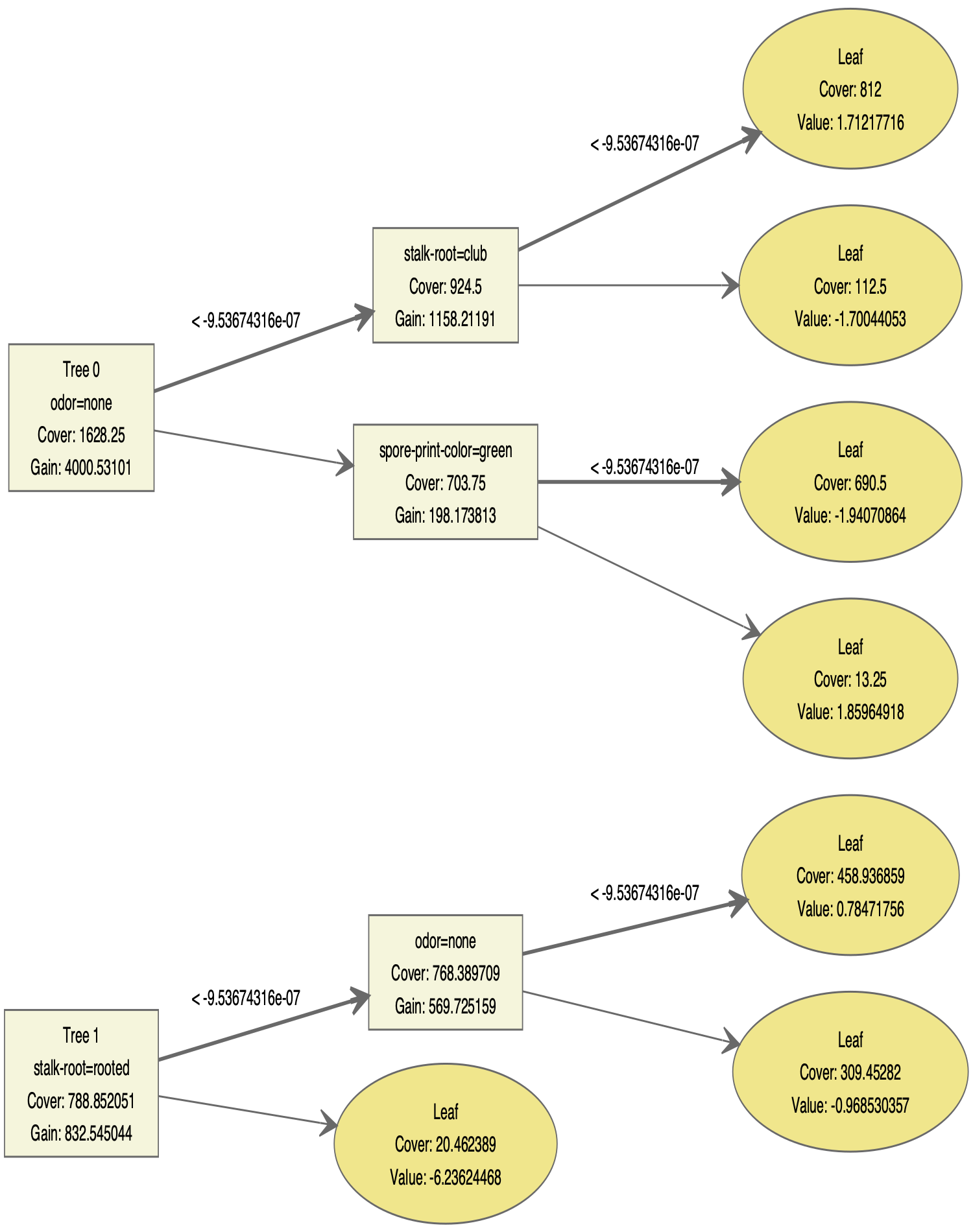

knitr::include_graphics(here::here("output/tree.png"))

10 保存模型

xgb.save(bst, here::here("output/xgboost.model"))

## [1] TRUE

# load binary model to R
bst2 <- xgb.load(here::here("output/xgboost.model"))
pred2 <- predict(bst2, test$data)

# And now the test
print(paste("sum(abs(pred2-pred))=", sum(abs(pred2-pred))))

## [1] "sum(abs(pred2-pred))= 0"

证明重新导入模型，没有问题！

但是我建议使用write_rds。

11 通过 SQL 部署

目前可以使用包 add2xgb 进行翻译。

翻译成SQL方便上线。

SQL逻辑见 mtcars_model_code.sql
通过可视化，可以确认自己的模型无误。见 visual_tree.Rmd
通过使用SQL和 predict 函数进行预测值的比较，发现无误。见 predictinsql.Rmd
本文的翻译函数参考rviews。但实际上函数是有些 typo 问题的，因此推荐阅读这个汉化版本。

我推荐，如果要工程化 Xgboost 的翻译，我建议学习 Xgboost 的底层逻辑。

每个 split 有三种状态，Yes、No 和 Missing
等等

当然，这个例子也可以帮助大家理解 Xgboost。

下一步，

我也将继续学习，在 data.frame 中进行树模型的学习，见 treestrintbl.Rmd

如上例子的代码可以参考 mtcars_xgboost.Rmd

12 翻译XGB线性学习器为方程

线性学习器完全是线性相加，因此约等于 OLS。参考讨论。

library(xgboost)
library(tidyverse)

train_data <- mtcars %>% 
    rename(y = am)
train_data[1,1]<- NA
anyNA(train_data) # 查看空值训练时被掠过，实际影响是什么？(被替代为0)

## [1] TRUE

dtrain <- 
    xgb.DMatrix(
        data = as.matrix(
            train_data %>% select(-y)
        )
        ,label = train_data$y
    )

base_score <- 
    mean(train_data$y)
    # 0.5
objective_i <- 
    "binary:logistic"
    # "reg:linear"
xgb_model <- xgb.train(
    params = list(booster = 'gblinear'),
    data=dtrain,
    nround=100,
    seed = 1, 
    max_depth = 1,
    objective = objective_i,
    base_score = base_score,
    verbose = 2
)

model_trees <- jsonlite::fromJSON(
    xgb.dump(xgb_model, with_stats = FALSE, dump_format='json'), 
    simplifyDataFrame = FALSE)

model_trees

## [[1]]
## [[1]]$bias
## [1] -0.866004
## 
## [[1]]$weight
##  [1]  0.05293380 -0.38562100 -0.02825550  0.03049800  1.09193000 -2.70359000
##  [7] -0.00780062 -4.40209000  2.56295000  0.03560790

yhat_auto <- xgb_model %>% predict(newdata = dtrain)

bias <- model_trees[[1]]$bias
weight_list <- model_trees[[1]]$weight
train_matrix <- train_data[!(names(train_data) %in% 'y')] %>% as.matrix()
dim(train_matrix)

## [1] 32 10

beta_matrix <-
    matrix(
        rep(weight_list, nrow(train_matrix)),
        ncol = ncol(train_matrix),
        nrow = nrow(train_matrix),
        byrow = TRUE
    )

yhat_raw <- (
     train_matrix * beta_matrix
) %>% rowSums(na.rm = TRUE) + bias +
    log(base_score/(1-base_score))
                     
# yhat_raw
yhat_man <- 1/(1+exp(-yhat_raw))
yhat_man

##           Mazda RX4       Mazda RX4 Wag          Datsun 710      Hornet 4 Drive 
##        9.379429e-01        9.582521e-01        8.670799e-01        1.994497e-04 
##   Hornet Sportabout             Valiant          Duster 360           Merc 240D 
##        1.644127e-03        1.320272e-04        8.902511e-03        7.037680e-02 
##            Merc 230            Merc 280           Merc 280C          Merc 450SE 
##        2.394308e-01        6.310021e-02        5.859964e-02        3.150566e-03 
##          Merc 450SL         Merc 450SLC  Cadillac Fleetwood Lincoln Continental 
##        8.229907e-03        6.424589e-03        7.029902e-07        9.038354e-07 
##   Chrysler Imperial            Fiat 128         Honda Civic      Toyota Corolla 
##        5.037606e-06        9.505864e-01        9.937041e-01        9.873432e-01 
##       Toyota Corona    Dodge Challenger         AMC Javelin          Camaro Z28 
##        1.760979e-01        1.118132e-03        3.131905e-03        9.549513e-03 
##    Pontiac Firebird           Fiat X1-9       Porsche 914-2        Lotus Europa 
##        1.691972e-04        9.676830e-01        9.999430e-01        9.996504e-01 
##      Ford Pantera L        Ferrari Dino       Maserati Bora          Volvo 142E 
##        9.712884e-01        9.996950e-01        9.953896e-01        7.306373e-01

yhat_auto

##  [1] 9.379443e-01 9.582530e-01 8.670828e-01 1.994547e-04 1.644161e-03
##  [6] 1.320302e-04 8.902678e-03 7.037856e-02 2.394357e-01 6.310175e-02
## [11] 5.860118e-02 3.150635e-03 8.230082e-03 6.424729e-03 7.030071e-07
## [16] 9.038571e-07 5.037733e-06 9.505876e-01 9.937043e-01 9.873435e-01
## [21] 1.761016e-01 1.118154e-03 3.131975e-03 9.549725e-03 1.692006e-04
## [26] 9.676838e-01 9.999430e-01 9.996505e-01 9.712891e-01 9.996951e-01
## [31] 9.953896e-01 7.306427e-01

sum(round(yhat_man,3)!=round(yhat_auto,3))

## [1] 0

base score 的问题老生常谈，依然是 logit 函数转换即可，参考讨论。

附录

这里主要展示那些使用Xgboost过程中，遇到的问题。

12.1 损失函数

损失函数(人工智能爱好者社区 2018)为

\[L(\phi) = \sum_i l(\hat y_i , y_i) + \sum_k \Omega(f_k) \\ \text{where }\Omega(f) = \gamma T + \frac{1}{2} \lambda ||w||^2\]

这里

$\sum_i l(\hat y_i , y_i)$ 衡量预测误差
$\sum_k \Omega(f_k)$ 衡量模型复杂程度
- $T$代表Nodes 的个数
- $w$代表节点的数值

12.2 最优化策略

考虑一个节点的情况(人工智能爱好者社区 2018)

\[w = \hat y\]

因此

\[L(\phi) = \sum_i l(w , y_i) + \sum_k \Omega(f_k) \\ \text{where }\Omega(f) = T + \frac{1}{2} \lambda ||w||^2\]

上述是一个关于$w$的一元二次方程，一阶导求解$w^*$。

12.3 Weighted Quantile Sketch

对于连续变量确定最佳分裂点时，如果唯一值超过一百，需要循环100次，这样运行时间很长，因此这里采用的方式是先虚拟化，利用二阶导数作权重，这里之后再详谈。

12.4 `gamma`参数

根据人工智能爱好者社区 (2018) 和 Foster (2015) 的描述$gamma$为 xgboost中分裂节点的增益函数

\[\mathrm{L_{split}} = \frac{1}{2}[\frac{(\sum_{i \in I_L}g_i)^2}{(\sum_{i \in I_L}h_i)^2 + \lambda} + \frac{(\sum_{i \in I_R}g_i)^2}{(\sum_{i \in I_R}h_i)^2 + \lambda} - \frac{(\sum_{i \in I}g_i)^2}{(\sum_{i \in I}h_i)^2 + \lambda}]-\gamma\]

增益函数是根据损失函数的下降值来计算，

\[\frac{(\sum_{i \in I_L}g_i)^2}{(\sum_{i \in I_L}h_i)^2 + \lambda}\]

衡量左边分裂后节点的损失值。 (L - left)

\[\frac{1}{2}[\frac{(\sum_{i \in I_R}g_i)^2}{(\sum_{i \in I_R}h_i)^2 + \lambda}\]

衡量右边分裂后节点的损失值。 (R - right)

\[\frac{1}{2}[\frac{(\sum_{i \in I}g_i)^2}{(\sum_{i \in I}h_i)^2 + \lambda}]\]

衡量未分裂前的损失值 ($I = I_L \bigcup I_R$)

因此三者之间的差距为损失函数的下降值，作为该split的信息增益。

$\gamma > 0$作为显著性水平的控制，之前的信息增益需大于$\gamma$才允许切分，因此$\gamma$起到了正则化的效果，控制了分裂次数，与lasso 和 ridge 等(见 lasso 的理解)控制$\beta$数量的思想类似。

12.5 Xgboost 处理缺失值的方式

Chen and Guestrin (2016 Section 3.4)给出了Xgboost自动处理缺失值的方式，相关分析见胡慧琦; 杨旭东; huanglk 。³ Xgboost不会覆盖缺失值，而是在每个节点分裂时，分别把缺失值放在左右两侧，分别计算信息增益，以更高的一种作为这个节点缺失值的处理方法。

例如在一个节点上，分列前，有50个样本

$x_i = 1$有30个，以A代替
$x_i = 0$有10个，以B代替
$x_i \text{ is null}$有10个，以C代替

这里的处理是，分别计算$(A+C,B)$和$(A,B+C)$两种方式，哪一种信息增益高，缺失值就放在哪一边。假设这里$(A+C,B)$最优。

那么在另外一个节点会有新的情况，

$x_i = 1$有20个，以A代替
$x_i = 0$有20个，以B代替
$x_i \text{ is null}$有10个，以C代替

这里的处理是，分别计算$(A+C,B)$和$(A,B+C)$两种方式，哪一种信息增益高，缺失值就放在哪一边。假设这里是和$(A,B+C)$最优。

因此缺失值的划分，每一次都不一样。因此缺失值在自动处理中，每个节点需要经过不同的pre-split 样本处理，因此达到了高性能的处理缺失值的方式（多个变量的参与）。

12.6 XGBoost可以自动处理缺失值

i.e. features that are not presented in the sparse feature matrix are treated as ‘missing’. XGBoost will handle it internally and you do not need to do anything on it.

Internally, XGBoost will automatically learn what is the best direction to go when a value is missing. Equivalently, this can be viewed as automatically “learn” what is the best imputation value for missing values based on reduction on training loss.

For continuous features, a missing(default) direction is learnt for missing value data to go into, so when the data of the speficific value is missing, then it goes to the default direction. (Chen 2014)

~~所以训练组要足够大，因为要防止一种风险，就是训练组没有NA，但是测试组有，这个不利于生产。~~

和 topic 不是很相关。

在 SQL 翻译时，我们会发现有三种结果 Yes No 和 Missing，最后一种对应了XGBoost自动处理缺失值的结果。可以使用xgb.dump观察。

Xgboost 不需要增加异常情况的处理相关 Issue https://github.com/JiaxiangBU/tutoring/issues/61#issuecomment-500192146

目前在 SQL 进行跑动模型时，分类变量都转换成连续变量，因此只需要考虑连续变量的情况。

每个变量的每个 case when 都有三种情况，>、<和NULL，因此在生产上任何一个变量出现 NULL，模型不会受到影响。

12.7 快速的变量重要性检验方式

Xgboost 可以不需要处理缺失值，见 12.6。

因此Xgboost 比随机森林更少减少人工对缺失值的干扰。
Xgboost 处理相关性特征变量，不会受到像随机森林一样的稀释作用 (diluted effect) ，具体见 Importances 数学定义。
相比较于其他的距离函数，基于树模型不是基于距离的模型，可以处理不同范围的特征。因此，建立树模型时不需要缩放。(Asaithambi 2019)

train <- read_csv("https://jiaxiangbu.github.io/picbackup/train.csv")
test <- read_csv("https://jiaxiangbu.github.io/picbackup/test.csv")
train$Name[1] <- NA
test$Name[1] <- NA
data1 <- bind_rows(train,test) %>% 
    filter(!is.na(Survived))

Xgboost manages only numeric vectors. (Tianqi Chen 2018)

Xgboost 只能进入连续变量，因此需要对分类变量进行one-hot。

data2 <- 
    data1 %>% 
    select(-PassengerId) %>% 
    select(Survived,Pclass,Sex,Age,SibSp,Parch,Sex,Embarked) %>% 
    mutate_if(is.character,~as.integer(as.factor(.))) %>% 
    select_if(~n_distinct(.,na.rm = T)>1)
    # 有些虽然有两个level，但是是NA和一个level，在dummyVars中要报错。

对于 category 变量直接转换为 ordinal。
1. 这样xgboost importances也会把分类变量的重要性归为一个变量，而不是分level。
2. 如果要单看level的重要性，也是可以看的。

# data3 <- 
# bind_cols(
# dummyVars(data2 %>% 
#   summarise_all(is.numeric) %>% 
#   gather() %>% 
#   filter(value == FALSE) %>%
#   .$key %>% 
#   paste(., collapse = "+") %>% 
#   paste("~",.),
# data = data2,
# fullrank = TRUE) %>% 
#   predict(.,newdata = data2) %>% 
#   as.tibble()
# ,
# data2 %>% 
#   select_if(is.numeric)  
# ) %>% 
#   select(Survived,everything())
data3 <- data2

data4 <- 
    xgb.DMatrix(
        data = as.matrix(data3 %>% select(-Survived))
        ,label = data3$Survived
        )

bst <- xgb.train(data = data4
                 ,max.depth = 4, num_parallel_tree = 1000, subsample = 0.5, colsample_bytree =0.5, nrounds = 1, objective = "binary:logistic")

xgb.importance(feature_names = colnames(data4), model = bst)

12.8 sparse.model.matrix 的注意点

sparse.model.matrix会直接让空值的行去除，因此做xgboost模型的预处理时，不建议，这相当于没有使用xgboost对缺失值处理的优势。

library(data.table)
library(tidyverse)
data <- 
    data.table(
        a=c(1,2,NA)
        ,b=c(3,NA,4)
    ) %>%
    mutate_all(as.factor)
data %>% 
    Matrix::sparse.model.matrix(a ~.-1,data=.)

## 1 x 2 sparse Matrix of class "dgCMatrix"
##   b3 b4
## 1  1  .

data %>% 
    as.matrix()

##      a   b  
## [1,] "1" "3"
## [2,] "2" NA 
## [3,] NA  "4"

在 Stack Overflow 上，我Post 一个答案，sparse.model.matrix函数会让有缺失值的行被剔除。

12.9 交叉项

The decision tree is a powerful tool to discover interaction among independent variables (features). (DMLC 2018)

When the tree depth is larger than one. (DMLC 2018)

booster [default= gbtree ]: Which booster to use. Can be gbtree, gblinear or dart; gbtree and dart use tree based models while gblinear uses linear functions.

gbtree 可以自动产生交叉项。

12.10 `logloss`评估

bst <- xgb.train(data=dtrain, 
                 max.depth=2, 
                 eta=1, 
                 nthread = 2, 
                 nround=2, 
                 watchlist=watchlist, 
                 eval.metric = "error", 
                 eval.metric = "logloss", 
                 objective = "binary:logistic")

## [1]  train-error:0.517887    train-logloss:0.954665  testhaha-error:0.518312 testhaha-logloss:0.955272 
## [2]  train-error:0.517887    train-logloss:0.733254  testhaha-error:0.518312 testhaha-logloss:0.733462

eval.metric = "error", eval.metric = "logloss"两个都加啊，别忘了。

12.11 install xgboost on Mac in python 2

Mac上就安装anacoda 的 py-xgboost 包，python 2 检测可以使用，代码直接

import xgboost

12.12 xgboost 和 lightBGM 的区别

阅读 Ke et al. (2017), Microsoft Corporation (2018) 后，会发现 lightBGM 和 xgboost 在性能上差不多，但是要快一些，这里主要讲讲区别。

12.12.1 深度 vs. 叶子数

lightBGM使用的是Leaf-wise (Best-first) Tree Growth，也就是对于每个树，优先增加叶子数，直观体现是深度，因此这样容易过拟合，因此调整参数的时候，深度的重要性上升。

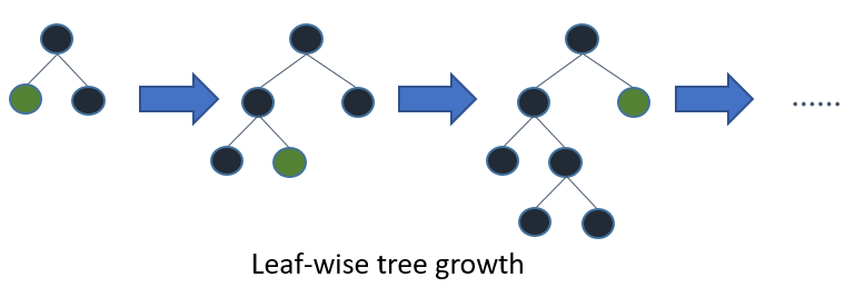
然而xgboost是level (depth)-wise的，也就是说平衡的增加深度，而不会出现某一个分支非常深。

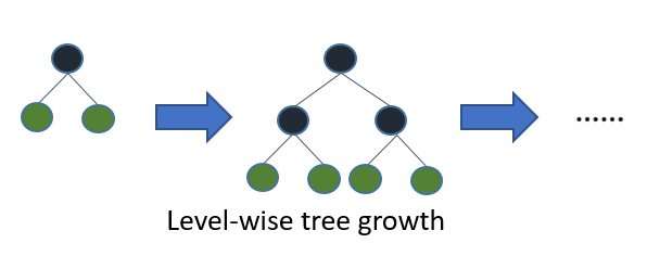
但是就是这点优化，使得每一次决策树不需要每一层都平衡的跑节点，这大大节省了时间，以为每一层的增加是指数级别的增加$2^k$，因此大大节省了时间。

除此之外，这是 GBDT的一个介绍PPT，知乎上的讨论也不少。

参考文献

Asaithambi, Sudharsan. 2019. “特征归一化.” 量化投资与机器学习. 2019. https://mp.weixin.qq.com/s/lyC1-scAzaPzBwtF50tPAA.

Brownlee, Jason. 2016. “Data Preparation for Gradient Boosting with Xgboost in Python.” 2016. https://machinelearningmastery.com/data-preparation-gradient-boosting-xgboost-python/.

Chen, Tianqi. 2014. “What Are the Ways of Treatng Missing Values in Xgboost?” 2014. https://github.com/dmlc/xgboost/issues/21.

Chen, Tianqi, and Carlos Guestrin. 2016. “XGBoost: A Scalable Tree Boosting System.” In ACM Sigkdd International Conference on Knowledge Discovery and Data Mining, 785–94.

Chen, Tianqi, Tong He, and Michaël Benesty. 2018. “Xgboost Presentation.” 2018. https://cran.r-project.org/web/packages/xgboost/vignettes/xgboostPresentation.html#view-feature-importanceinfluence-from-the-learnt-model.

DMLC. 2016a. “Understand Your Dataset with Xgboost.” 2016. http://xgboost.readthedocs.io/en/latest/R-package/discoverYourData.html.

———. 2016b. “XGBoost R Tutorial.” 2016. https://xgboost.readthedocs.io/en/latest/R-package/xgboostPresentation.html.

———. 2018. “Feature Interaction Constraints: XGBoost R Tutorial.” 2018. https://xgboost.readthedocs.io/en/latest/tutorials/feature_interaction_constraint.html.

Foster, David. 2015. “How Is Xgboost Quality Calculated?” 2015. https://stackoverflow.com/questions/33654479/how-is-xgboost-quality-calculated.

Ke, Guolin, Qi Meng, Thomas Finley, Taifeng Wang, Wei Chen, Weidong Ma, Qiwei Ye, and Tie-Yan Liu. 2017. “LightGBM: A Highly Efficient Gradient Boosting Decision Tree.” In Advances in Neural Information Processing Systems 30, edited by I. Guyon, U. V. Luxburg, S. Bengio, H. Wallach, R. Fergus, S. Vishwanathan, and R. Garnett, 3146–54. Curran Associates, Inc. http://papers.nips.cc/paper/6907-lightgbm-a-highly-efficient-gradient-boosting-decision-tree.pdf.

Microsoft Corporation. 2018. LightGBM. Microsoft Corporation. https://lightgbm.readthedocs.io/en/latest/Features.html.

Sandhu, Sandeep S. 2016. “How Do I Interpret the Output of Xgboost Importance?” 2016. https://datascience.stackexchange.com/questions/12318/how-do-i-interpret-the-output-of-xgboost-importance.

Srivastava, Tavish. 2016. “How to Use Xgboost Algorithm in R in Easy Steps.” Analytics Vidhya. 2016. https://www.analyticsvidhya.com/blog/2016/01/xgboost-algorithm-easy-steps/.

Tianqi Chen, Michaël Benesty, Tong He. 2018. “Understand Your Dataset with Xgboost.” 2018. https://cran.r-project.org/web/packages/xgboost/vignettes/discoverYourData.html#numeric-v.s.-categorical-variables.

人工智能爱好者社区. 2018. “通俗的将Xgboost的原理讲明白.” 2018. https://mp.weixin.qq.com/s/10trsyoH1ors-fzLsYjO3w.

~~Windows user will need to install Rtools first.~~ 最新版本似乎不需要了。↩
In a sparse matrix, cells containing 0 are not stored in memory. Therefore, in a dataset mainly made of 0, memory size is reduced. It is very usual to have such dataset. 因此非常适合 one hot 的数据。↩
In fact, XGBoost was designed to work with sparse data, like the one hot encoded data from the previous section, and missing data is handled the same way that sparse or zero values are handled, by minimizing the loss function. (Brownlee 2016)

Brownlee (2016) 分别试验了缺失值变为0,1,均值后得到验证，Xgboost识别为0的效果最好。因此缺失值除非有特别的业务逻辑，可以不做处理，Xgboost会找到最好的处理方式，但是感觉和@Chen2016XGBoost [Section 3.4]的主要意思不相关。↩

XGBoost using R 学习笔记

XGBoost using R 学习笔记

1 安装¹

2 数据导入

2.1 导入方式

2.2 xgb.DMatrix

3 配置信息查看 verbose

4 分类问题

5 回归问题

6 预测

7 从`xgb.DMatrix`中取出信息

8 特征重要性

8.1 理论

8.2 计算

9 导出树的结构

10 保存模型

11 通过 SQL 部署

12 翻译XGB线性学习器为方程

附录

12.1 损失函数

12.2 最优化策略

12.3 Weighted Quantile Sketch

12.4 `gamma`参数

12.5 Xgboost 处理缺失值的方式

12.6 XGBoost可以自动处理缺失值

12.7 快速的变量重要性检验方式

12.8 sparse.model.matrix 的注意点

12.9 交叉项

12.10 `logloss`评估

12.11 install xgboost on Mac in python 2

12.12 xgboost 和 lightBGM 的区别

12.12.1 深度 vs. 叶子数

参考文献

XGBoost using R 学习笔记

1 安装1

2 数据导入

2.1 导入方式

2.2 xgb.DMatrix

3 配置信息查看 verbose

4 分类问题

5 回归问题

6 预测

7 从xgb.DMatrix中取出信息

8 特征重要性

8.1 理论

8.2 计算

9 导出树的结构

10 保存模型

11 通过 SQL 部署

12 翻译XGB线性学习器为方程

附录

12.1 损失函数

12.2 最优化策略

12.3 Weighted Quantile Sketch

12.4 gamma参数

12.5 Xgboost 处理缺失值的方式

12.6 XGBoost可以自动处理缺失值

12.7 快速的变量重要性检验方式

12.8 sparse.model.matrix 的注意点

12.9 交叉项

12.10 logloss评估

12.11 install xgboost on Mac in python 2

12.12 xgboost 和 lightBGM 的区别

12.12.1 深度 vs. 叶子数

参考文献

1 安装¹

7 从`xgb.DMatrix`中取出信息

12.4 `gamma`参数

12.10 `logloss`评估