使用 RMarkdown 的 child 参数，进行文档拼接。
这样拼接以后的笔记方便复习。
相关问题提交到 GitHub

本文于2020-10-23更新。如发现问题或者有建议，欢迎提交 Issue

线性代数可以算是机器学习的基础。线性代数的学习和复习我建议还找R或者Matlab，边跑边理解线性代数的一些特性和规则，这样比较形象直观。 R相关的例子，见 9.8。

无监督学习中的PCA的计算，底层使用到线性代数计算协方差矩阵，求解特征值等。
1. PCA方式也是展示大数据特征向量的方法之一，详见训练模型 training model 使用技巧的 PCA的展示方式

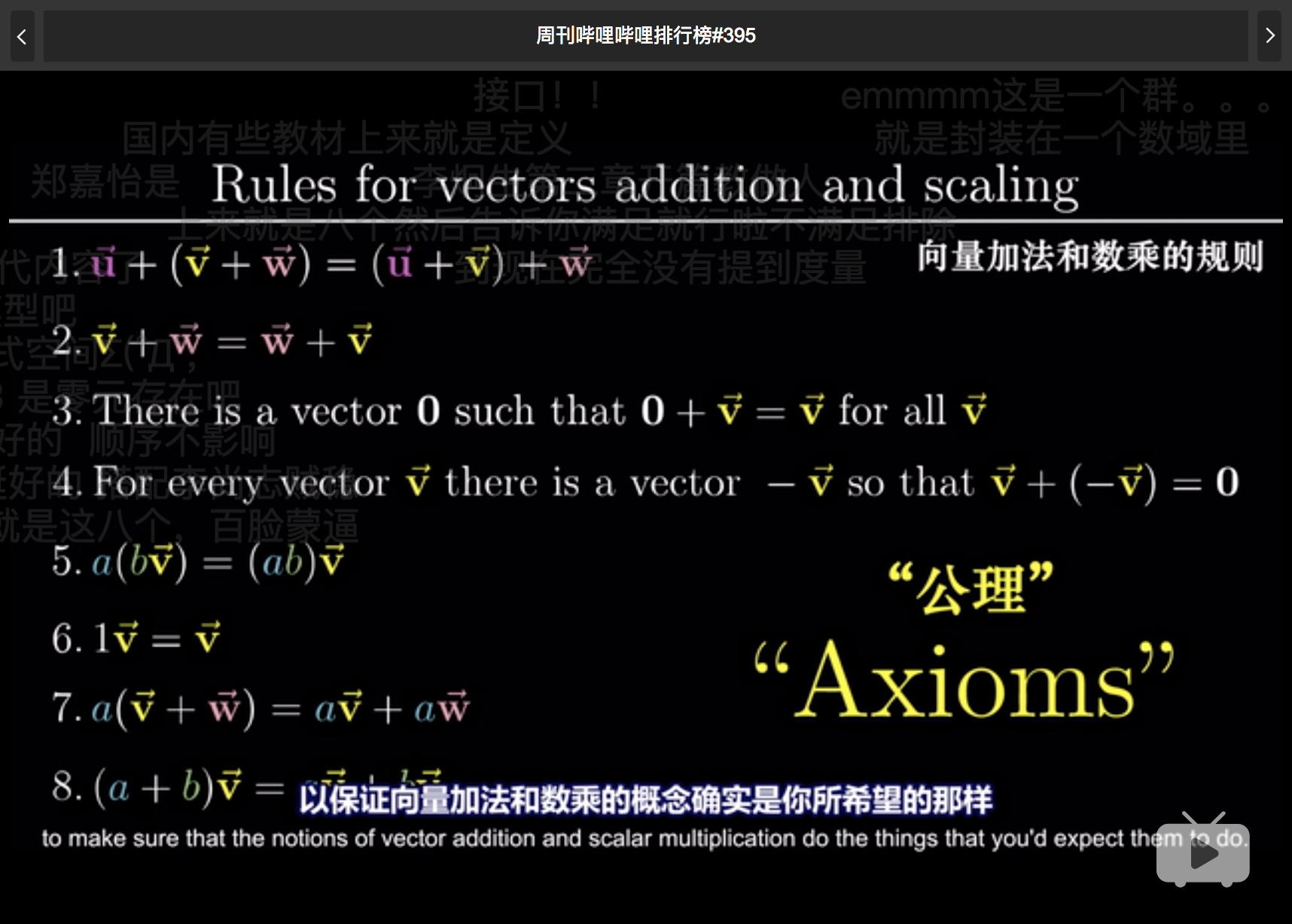
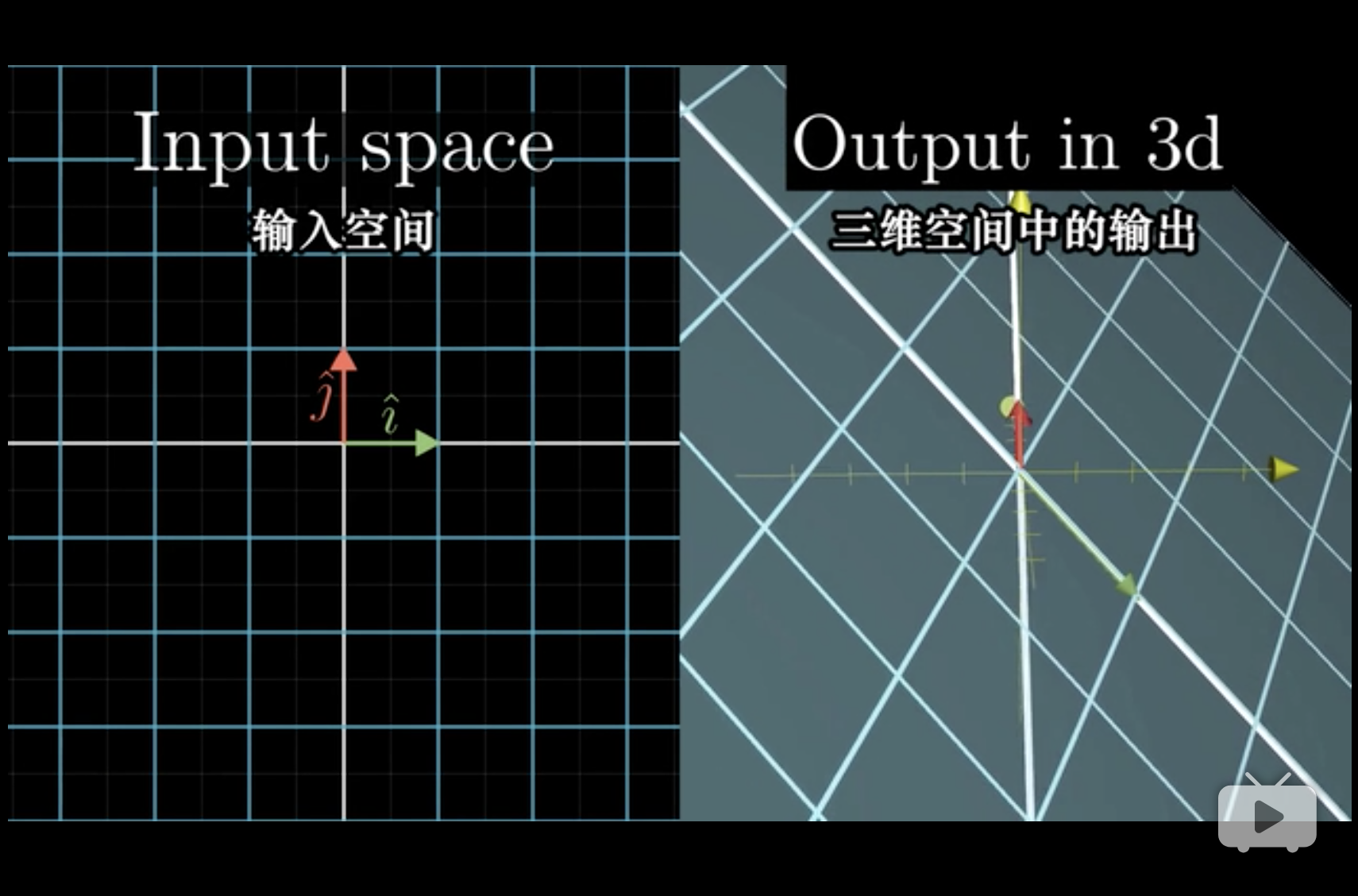
1 线性变换几何理解

线性变换 (linear transformation) 从几何理解来看，空间的拉伸和压缩。 (3Blue1Brown 2018, Edition 3) 在二维空间中，线性变换就是平面变换，原点不变。因为没有发生平移。线性变换很常见，常用于基变换，见 8。

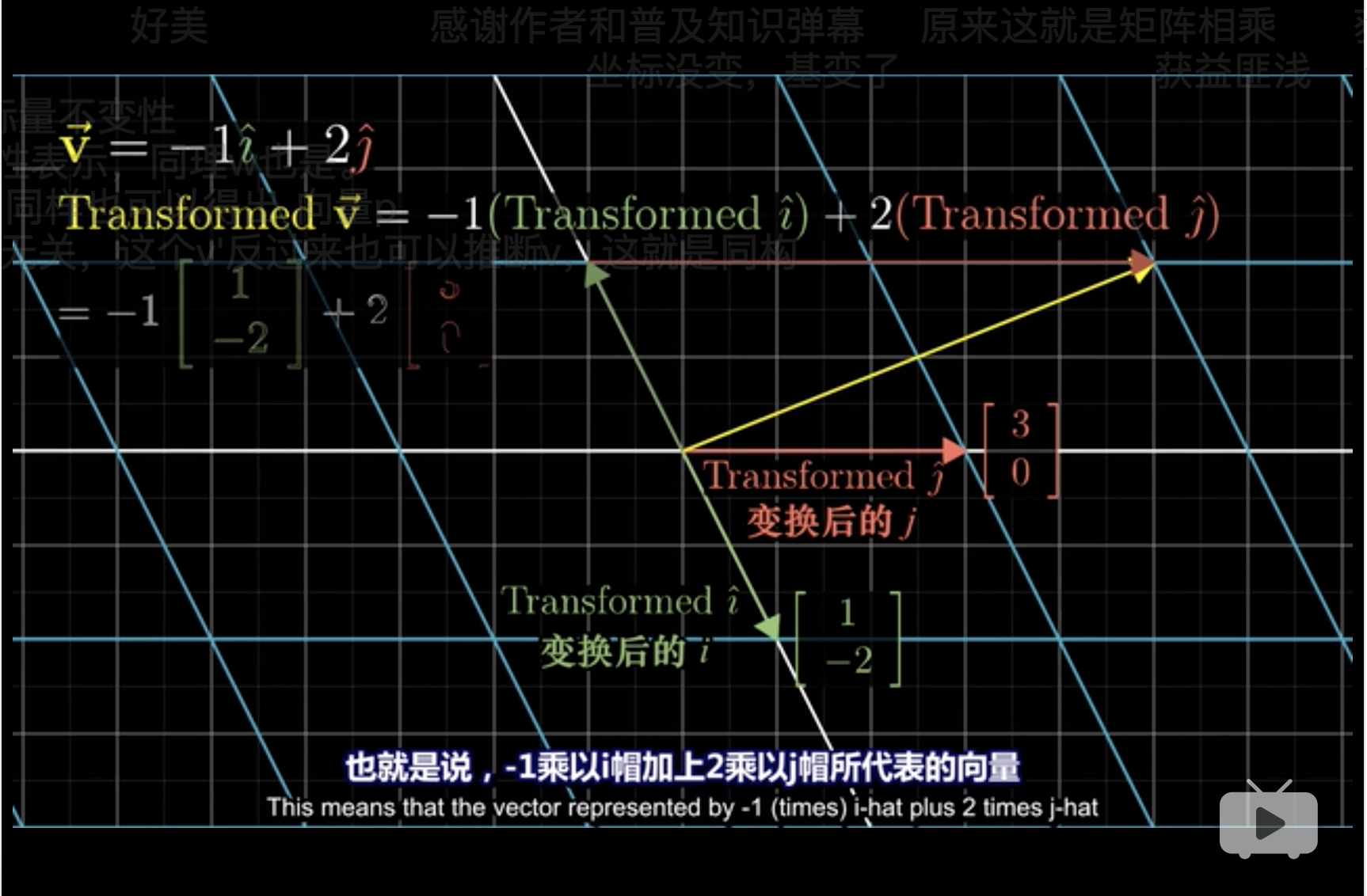
这里\(\vec{V} = -1 \hat i + 2 \hat j\)，无论平面如何变化，这个关系不变，但是当平面通过旋转发生改变后， \(i\)和\(j\)发生了改变。 \[i=\begin{bmatrix} 1 \\ -2 \\ \end{bmatrix}\]且 \[j=\begin{bmatrix} 3 \\ 0 \\ \end{bmatrix}\]

所以，

\[\vec{V} = -1\begin{bmatrix} 1 \\ -2 \\ \end{bmatrix} + 2\begin{bmatrix} 3 \\ 0 \\ \end{bmatrix} = \begin{bmatrix} -1(1) + 2(3) \\ -1(-2) + 2(0) \\ \end{bmatrix}\]

在R可以实现，

v <- matrix(c(-1,2),nrow = 2)
trans <- matrix(c(c(1,-2),c(3,0)),nrow=2,byrow = F)
trans

##      [,1] [,2]
## [1,]    1    3
## [2,]   -2    0

##      [,1]
## [1,]   -1
## [2,]    2

trans

##      [,1] [,2]
## [1,]    1    3
## [2,]   -2    0

diag(2)%*%v

##      [,1]
## [1,]   -1
## [2,]    2

trans%*%v

##      [,1]
## [1,]    5
## [2,]    2

trans[,1]*v[1]+trans[,2]*v[2]

## [1] 5 2

单位标准基diag(2)对v没有影响
trans改变了v在原平面的表达
trans的两列相当于两个基，v的两行对应两个基。

因此一半的，可以写成，

\[\begin{bmatrix} x \\ y \\ \end{bmatrix} \to x \begin{bmatrix} 1 \\ -2 \\ \end{bmatrix} + y\begin{bmatrix} 3 \\ 0 \\ \end{bmatrix} = \begin{bmatrix} 1x+3y \\ -2x+0y \end{bmatrix}\]

因此，

\[ \begin{bmatrix} 1 & 3 \\ -2 & 0 \\ \end{bmatrix} \begin{bmatrix} x \\ y \\ \end{bmatrix} = x \begin{bmatrix} 1 \\ -2 \\ \end{bmatrix} + y\begin{bmatrix} 3 \\ 0 \\ \end{bmatrix} \]

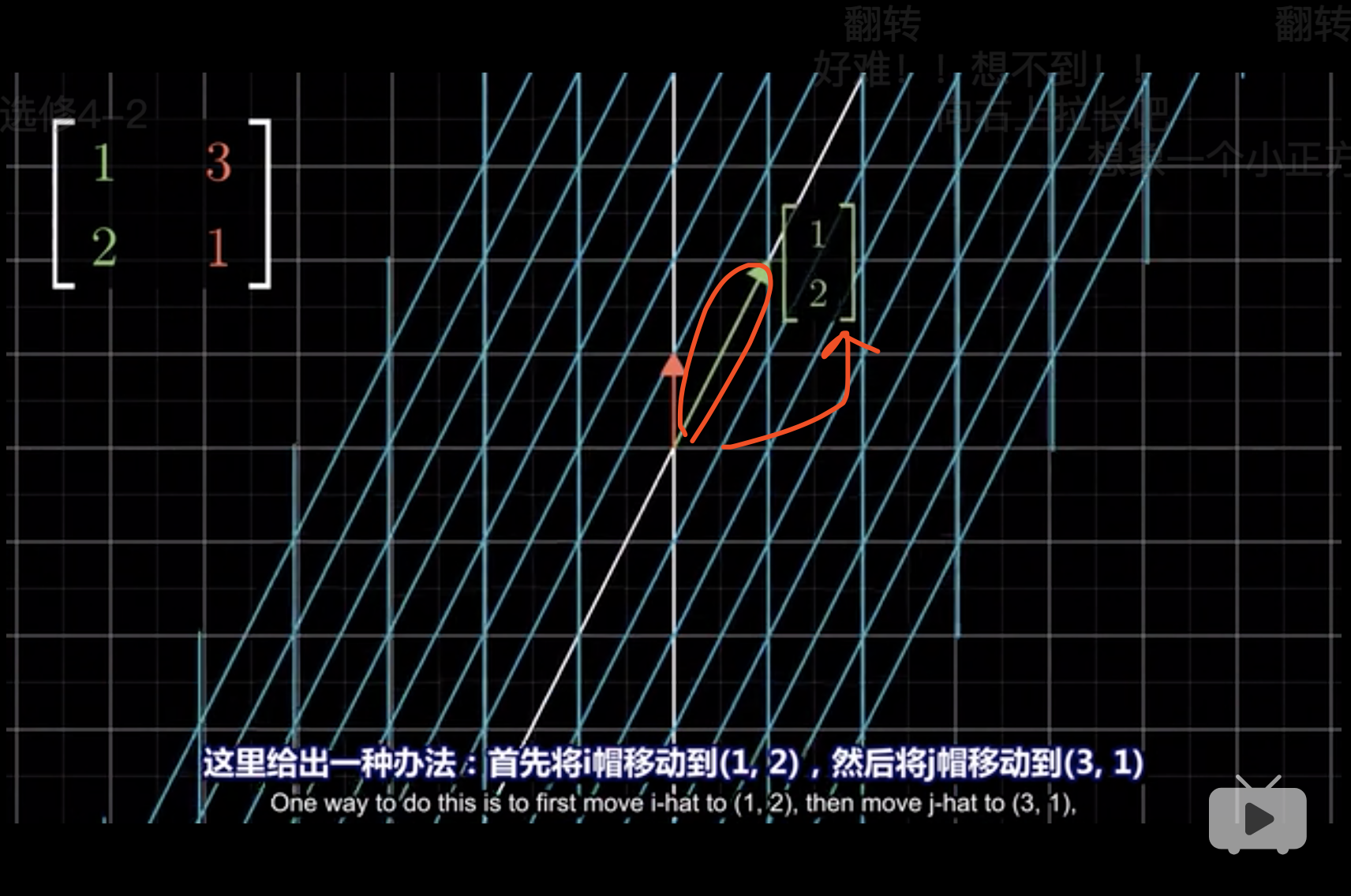
这种变化，就是把每个基的箭头看成一个点，

点\((1,0)\to(2,1)\)
然后平面翻转，点\((0,1)\to(3,1)\)

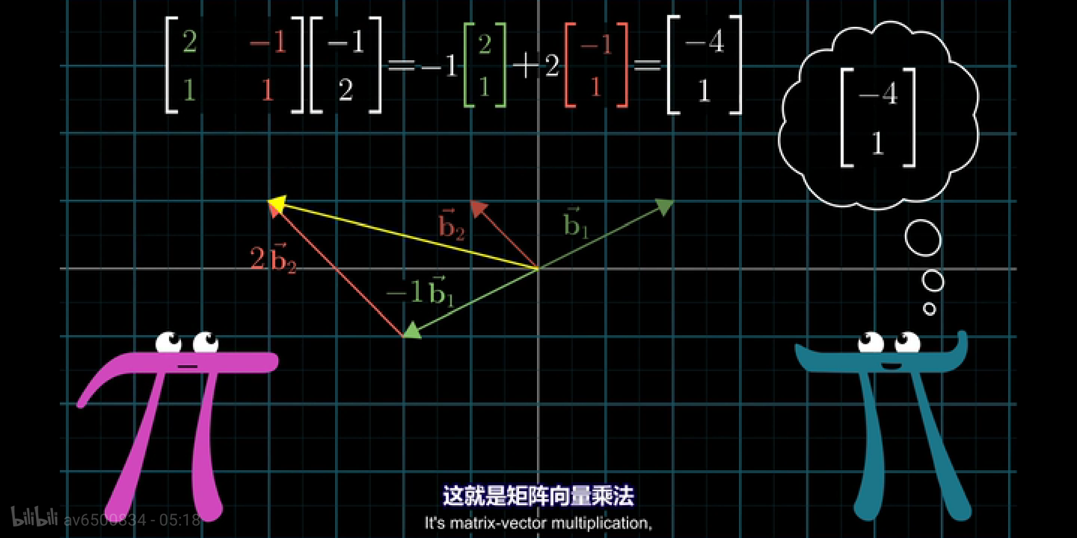
2 矩阵乘法理解

根据线性变换见 1，线性变化不改变原点的位置，但是压缩拉伸平面。压缩拉伸的效果完全由基决定。

接下来具体讨论矩阵乘法理解在几何上的理解。 (3Blue1Brown 2018, Edition 4)

在几何上，矩阵乘法理解可以认为是，\(\vec{A} \times \vec{B}\)

作为基，压缩拉伸空间
作为一组向量，被基进行变换位置，原点不动。

以下举一个具体的例子，\(M_1\)中的每个向量如何通过\(M_2\)进行变换。

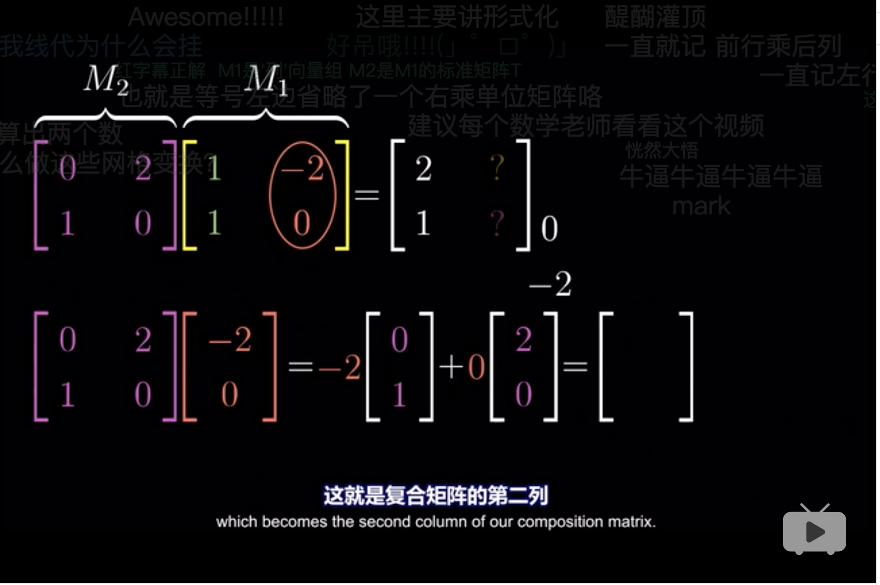
先将\(M_2\)中的\(\begin{bmatrix}0\\1\\ \end{bmatrix}\)看成一个基， \(\begin{bmatrix}0\\1\\ \end{bmatrix}\)和 \(M_1 = \begin{bmatrix}1 & -2 \\ 1 & 0 \\ \end{bmatrix}\)相乘
再将\(M_2\)中的\(\begin{bmatrix}2\\0\\\end{bmatrix}\)看成一个基， \(\begin{bmatrix}2\\0\\ \end{bmatrix}\)和 \(M_1 = \begin{bmatrix}1 & -2 \\ 1 & 0 \\ \end{bmatrix}\)相乘

具体在R=中的实现如下。

m2 <- matrix(c(0,2,1,0),nrow = 2,byrow = T)
m1 <- matrix(c(1,-2,1,0),nrow=2,byrow = T)
m2;m1

##      [,1] [,2]
## [1,]    0    2
## [2,]    1    0

##      [,1] [,2]
## [1,]    1   -2
## [2,]    1    0

diag(2)%*%m1;m2%*%m1

##      [,1] [,2]
## [1,]    1   -2
## [2,]    1    0

##      [,1] [,2]
## [1,]    2    0
## [2,]    1   -2

diag(2)[,1];m2[,1];diag(2)[,1]%*%m1;m2[,1]%*%m1

## [1] 1 0

## [1] 0 1

##      [,1] [,2]
## [1,]    1   -2

##      [,1] [,2]
## [1,]    1    0

diag(2)[,2];m2[,2];diag(2)[,2]%*%m2;m2[,2]%*%m1

## [1] 0 1

## [1] 2 0

##      [,1] [,2]
## [1,]    1    0

##      [,1] [,2]
## [1,]    2   -4

将基diag(2)[,1]替换成m2[,1]
将基diag(2)[,2]替换成m2[,2]

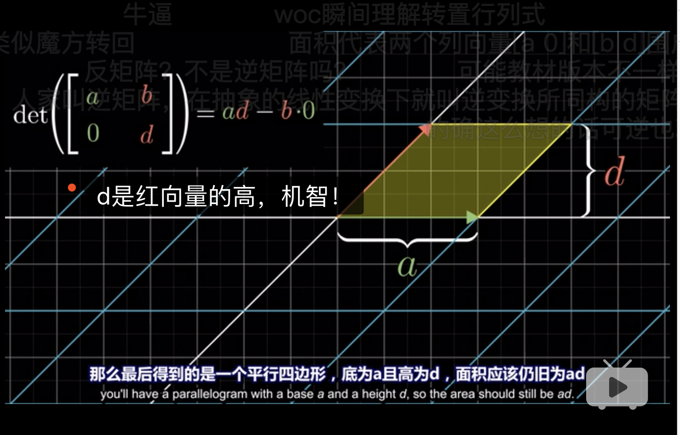
3 用面积理解行列式

在平面几何中行列式 (determinant) 表示两个向量形成的平行是四边形的面积。 (3Blue1Brown 2018, Edition 5)

为了直观，我们先假设两个向量在标准正交基上。

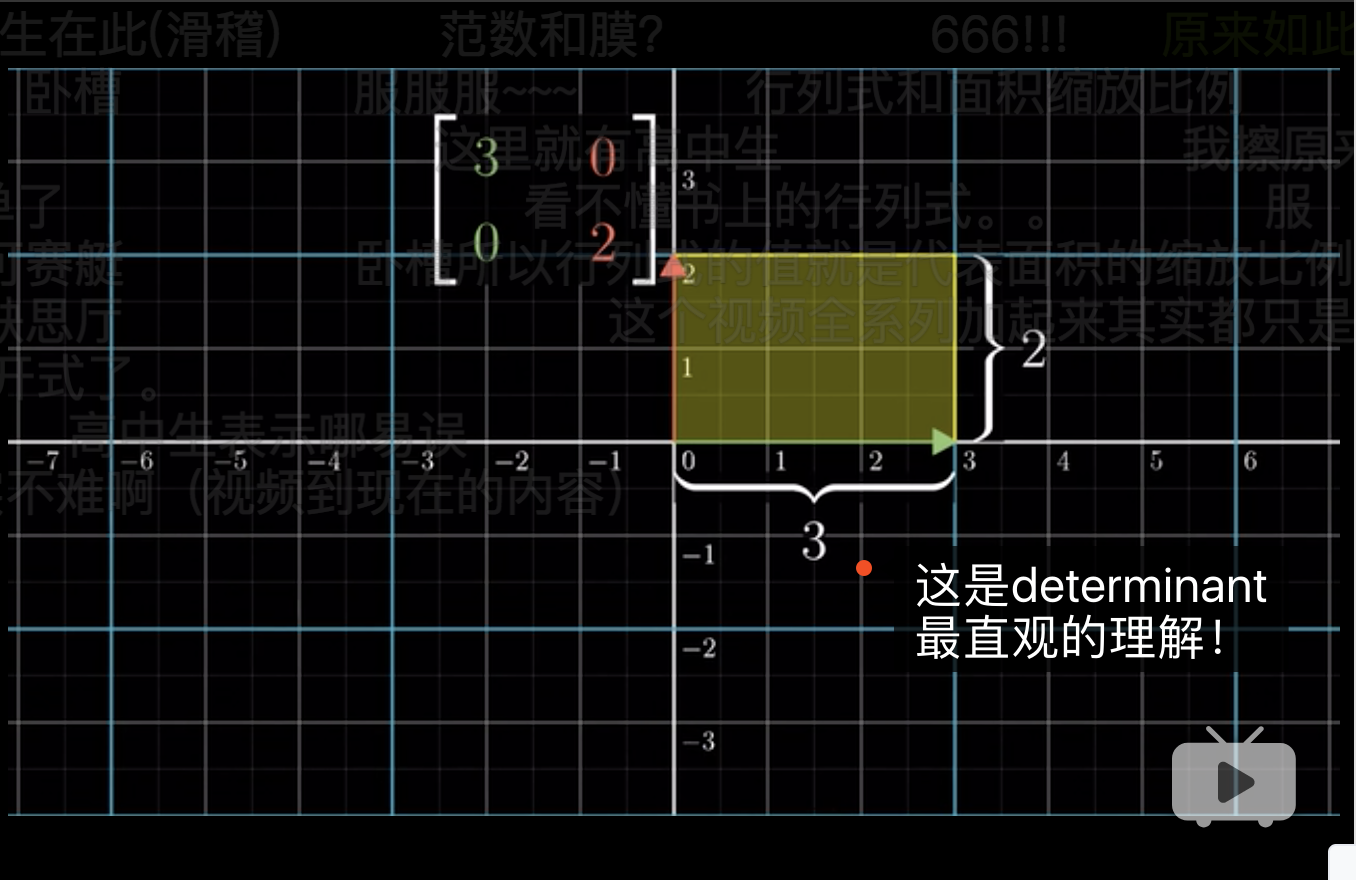
如图，在R中求解det，

some_mtr <- matrix(c(3,0,0,2),nrow = 2,byrow = T)
some_mtr

##      [,1] [,2]
## [1,]    3    0
## [2,]    0    2

det(some_mtr)

## [1] 6

3*2

## [1] 6

3.1 det < 0 的情况

some_mtr <- matrix(1:4,nrow = 2,byrow = T)
det(some_mtr)

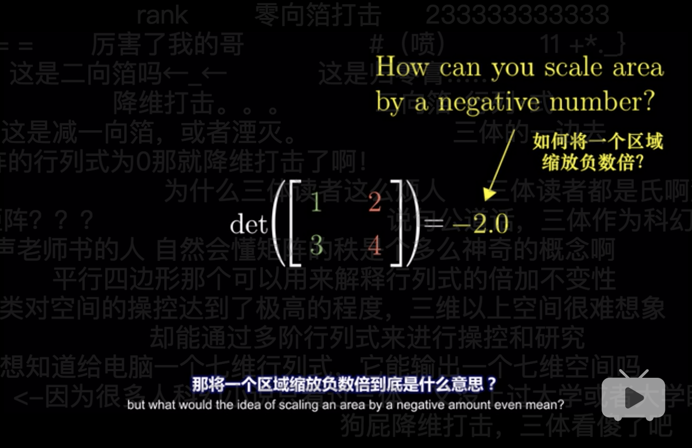
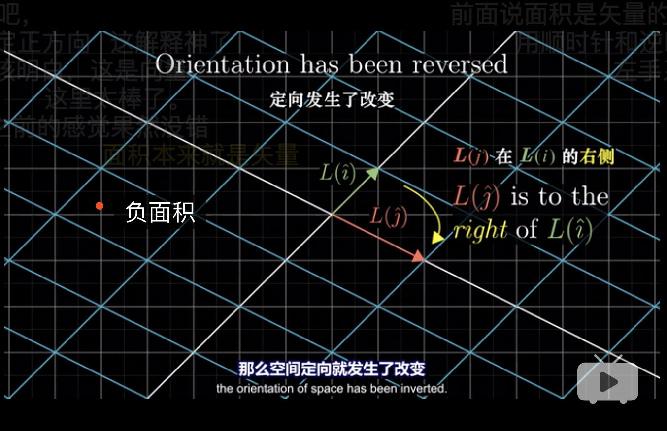
## [1] -2

这个是很好的把几何和代数联系在一起了。负面积就是线性变换见 1 时翻转平面，180度的旋转。

实现过程上是\(i\)和\(j\)互换位置。

可以在R中进行验证，

some_mtr[,c(2,1)]

##      [,1] [,2]
## [1,]    2    1
## [2,]    4    3

some_mtr[,c(2,1)] %>% det

## [1] 2

3.2 如何理解反转

因为首先正常\(\to\)反转的过程中，一个过渡状态就是\(i\)和\(j\)共线
在平面挤压过程中，就好像平面在进行翻面一样，因为要和原平面保持垂直时，\(i\)和\(j\)在原平面上的投影看起来才是一条线上。

3维中的flip，就可以理解这个正方形进行了原点对称。

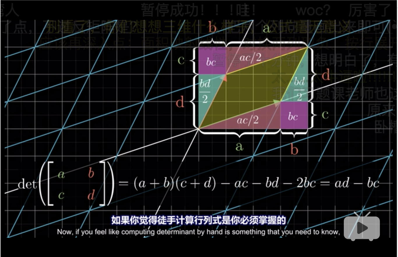
3.3 det 的计算公式推导

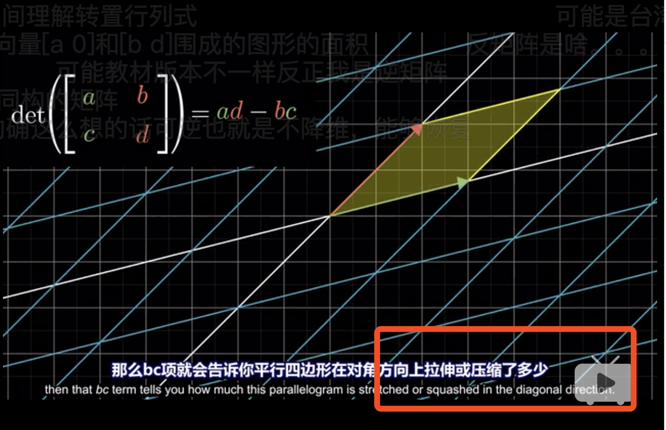
显然\(b\)和\(c\)衡量了红和绿向量向对角线的偏移，这导致了在计算面积时的高缩减了，因此这算是一种减少。

4 逆矩阵

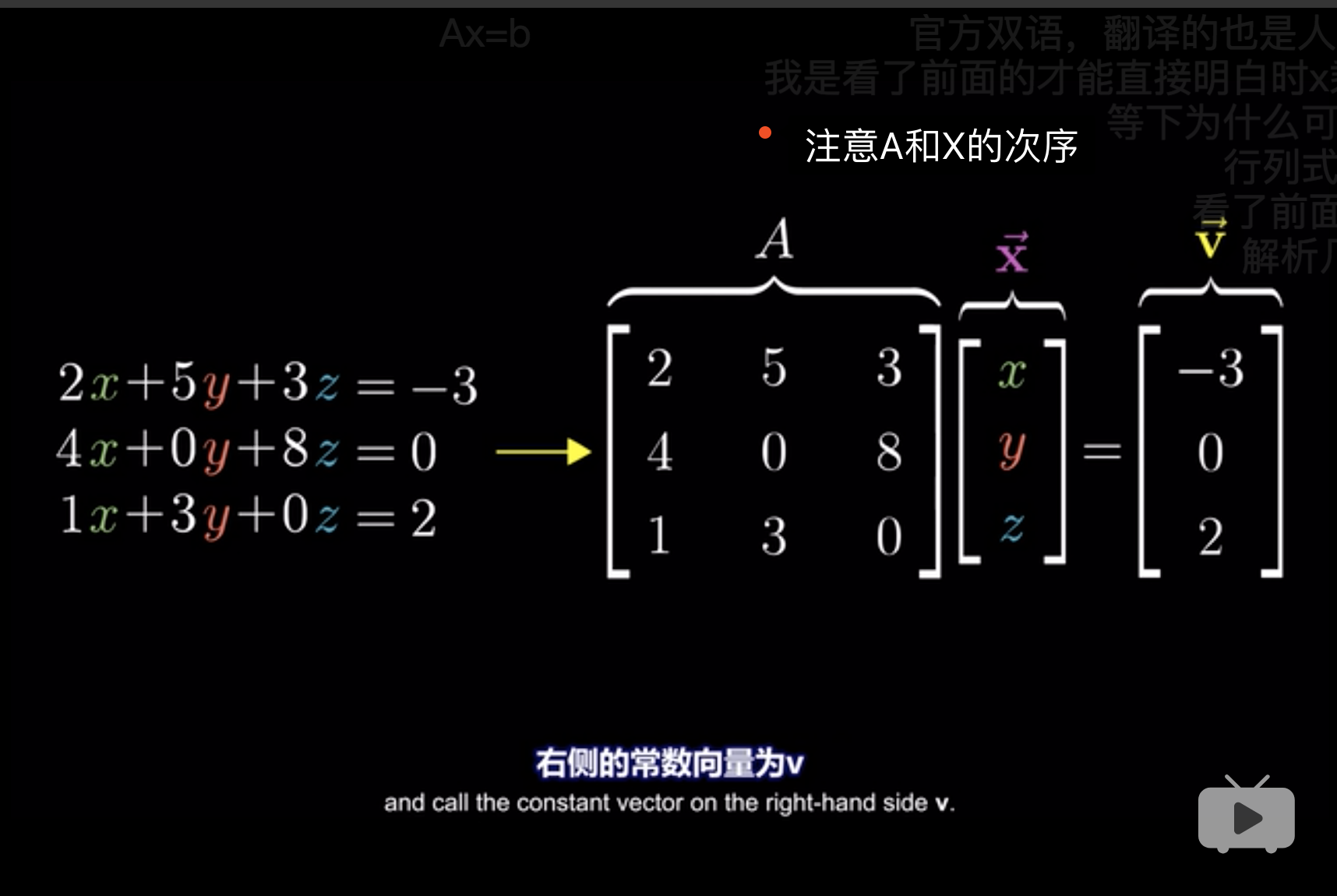
从几何角度，线性方程组可以理解为input \(x\)，作为基，
基是常数项形成的向量，
output就是右边的常数项形成的向量，
output就是根据线性变换后的结果。

在R中实现，方程组的求解。

params_mtr <- matrix(c(2,5,3,4,0,8,1,3,0),nrow = 3,byrow = 3)
y_mtr <- matrix(c(-3,0,2),nrow = 3)
params_mtr

##      [,1] [,2] [,3]
## [1,]    2    5    3
## [2,]    4    0    8
## [3,]    1    3    0

y_mtr

##      [,1]
## [1,]   -3
## [2,]    0
## [3,]    2

x <- solve(params_mtr)%*%y_mtr
x

##           [,1]
## [1,]  5.428571
## [2,] -1.142857
## [3,] -2.714286

solve用于求逆矩阵，参考 Eager (2018)

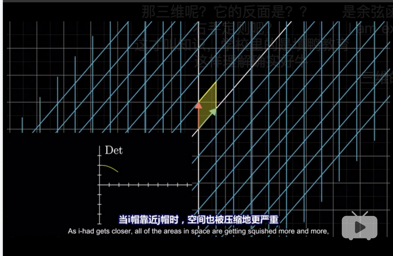
4.1 det(A) = 0

从几何意义上，\(\det(A) = 0\)

表示了面积为0，
相当于把一个二维向量压缩到了一个直线上，
这个时候，想要从一条直线返回到一个平面，存在无数种解，这就是不可逆。(3Blue1Brown 2018, Edition 6) 具体如下图，
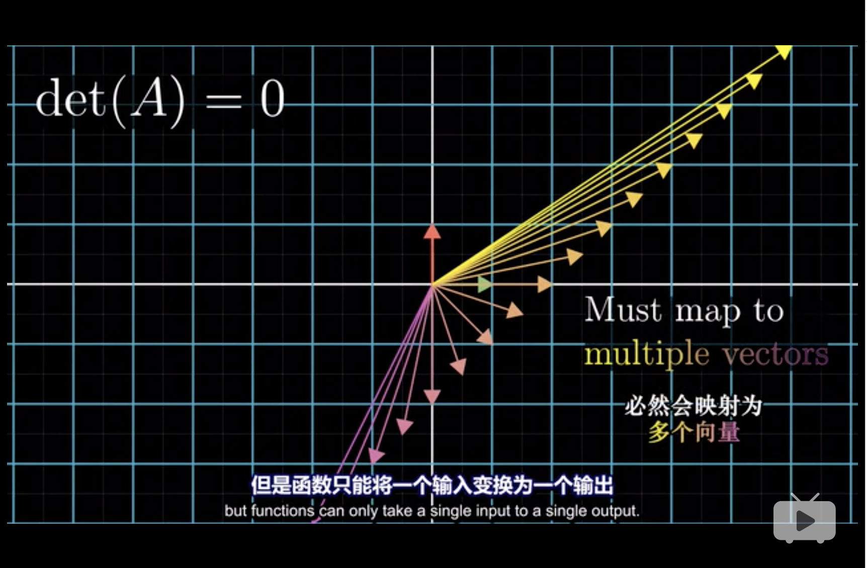
1. 对应地，代数中，\(0 \cdot x = 1\)中，\(x\)可以为任意数。

4.2 \(\det(A^{-1}A)=1\)

some_mtr <- matrix(1:4,nrow = 2,byrow = T)
some_mtr

##      [,1] [,2]
## [1,]    1    2
## [2,]    3    4

some_mtr %>% det

## [1] -2

some_mtr %>% solve

##      [,1] [,2]
## [1,] -2.0  1.0
## [2,]  1.5 -0.5

some_mtr %>% solve %>% det

## [1] -0.5

some_mtr %>% t

##      [,1] [,2]
## [1,]    1    3
## [2,]    2    4

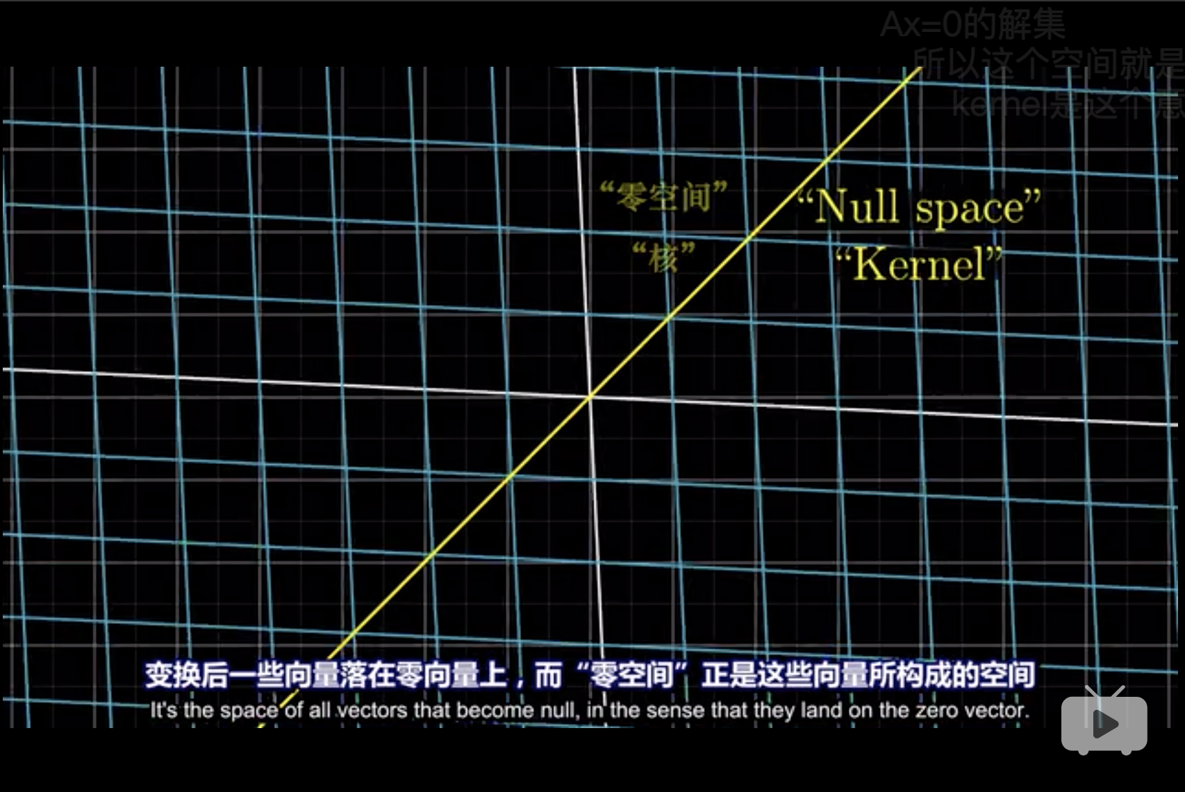
some_mtr %>% t %>% det

## [1] -2

5 列空间、秩与零空间

\[\text{rank}(\text{input}) \geq \text{rank}(\text{output})\]

那么，

\[\text{collapse} = \Delta \text{rank} = \text{rank}(\text{input}) - \text{rank}(\text{output})\]

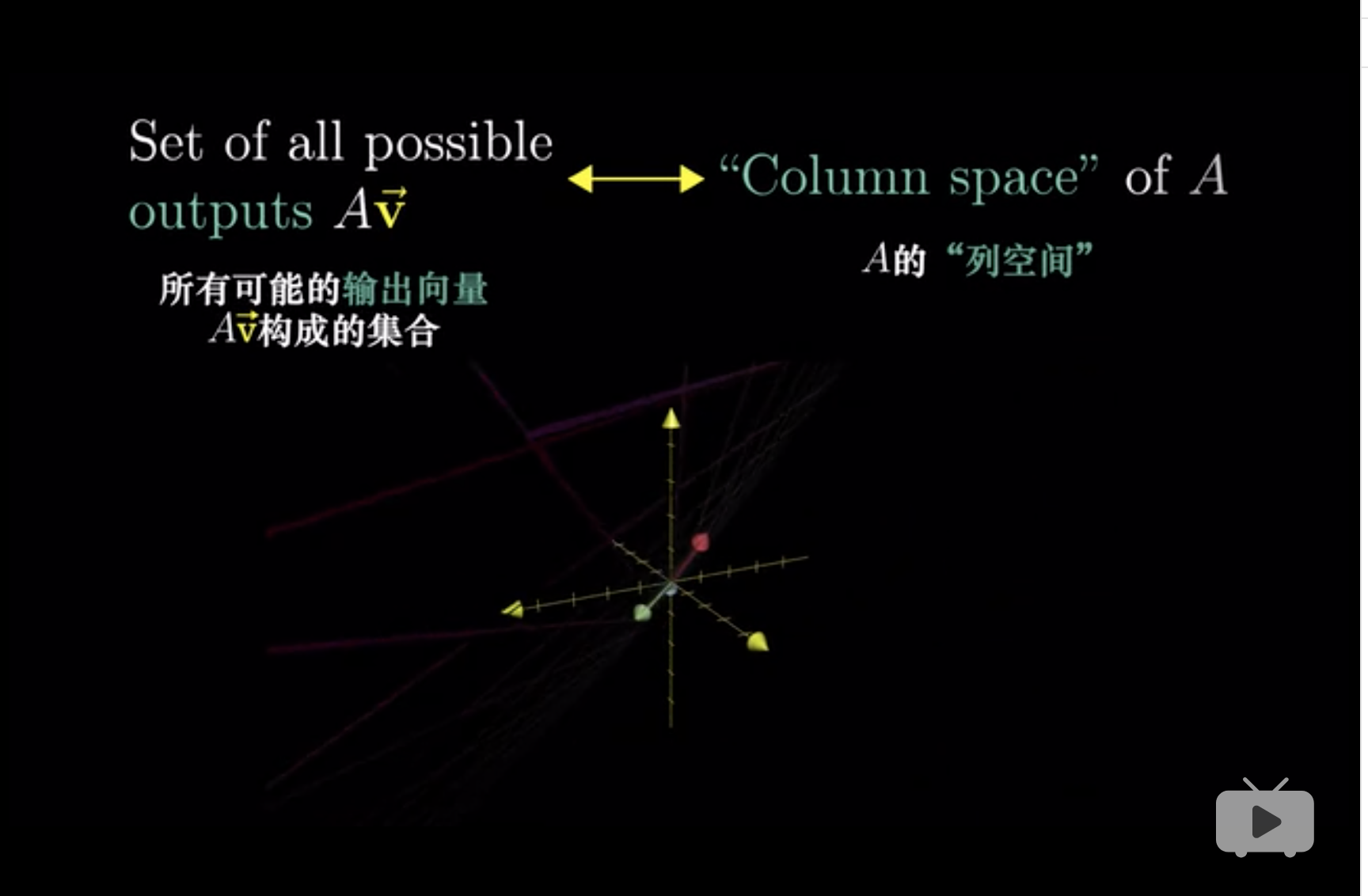
因此，那些被降维的向量，可以理解为某方向的分向量被压缩到了原点，这种操作的后果就是， null space or kernel。被降维的向量的选择是具备条件的，比如PCA，就是解释方差小的向量被舍弃了。 (3Blue1Brown 2018, Edition 6)

6 点积

从投影的理解方式看，

\[\vec{v}\cdot\vec{w}=|\vec{v}|\cdot|\vec{w}| \cdot \cos(\theta)\]

点积类似于\(\vec{w}\)向\(\vec{v}\)方向上的投影，计算为\(|\vec{w}| \cdot \cos(\theta)\)。

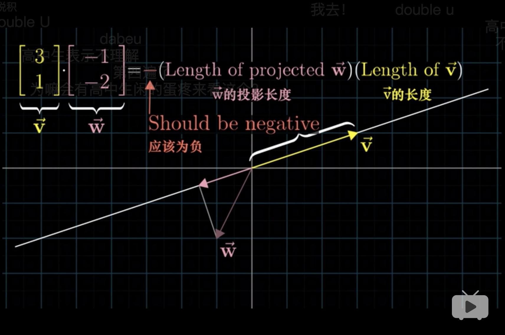
从几何的理解方式看，

从几何角度上，相当于先把\(\vec{w}\)压缩到\(\vec{v}\)上，原来二维空间的两个基被投影到了这条直线上了。

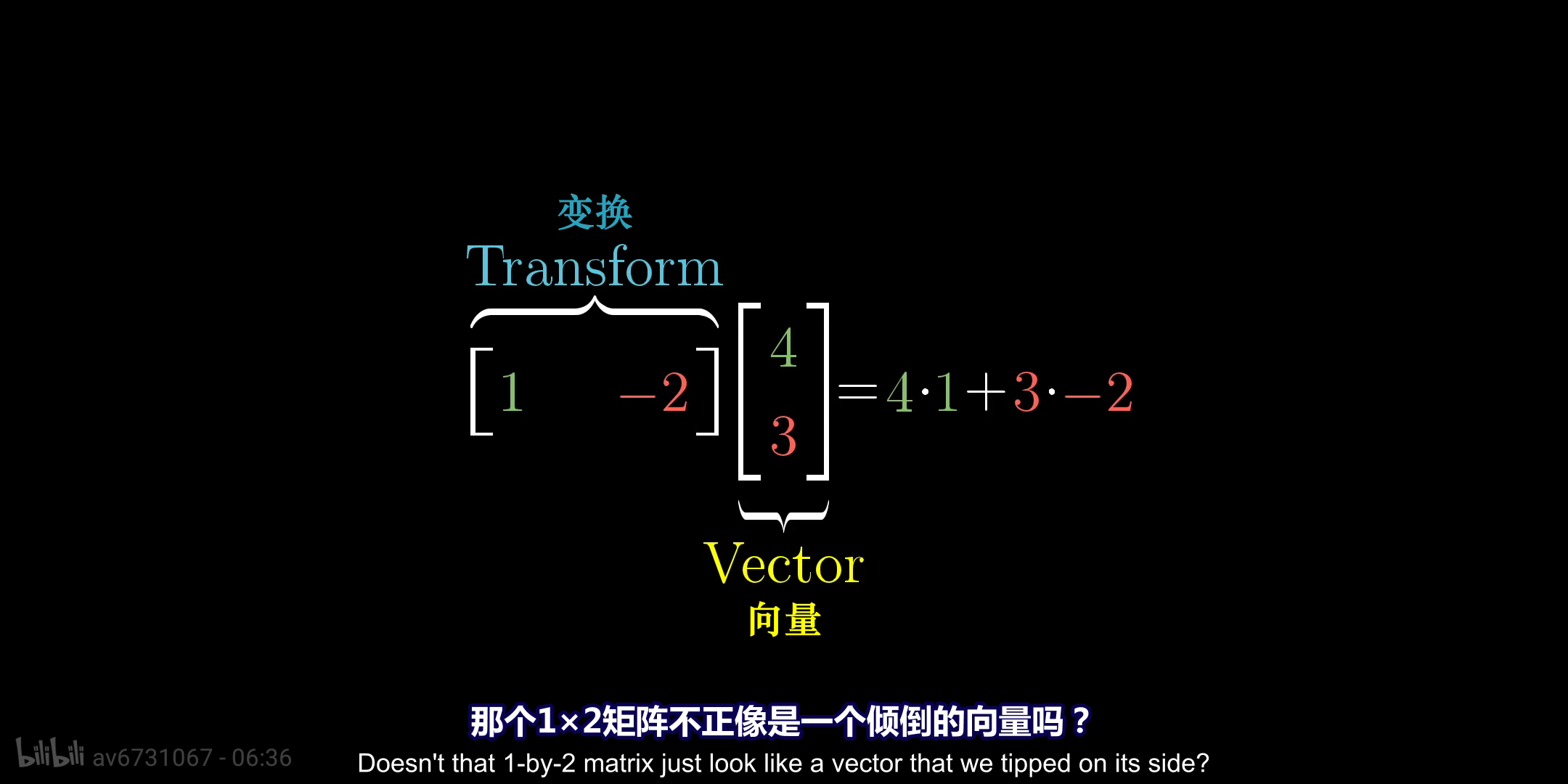
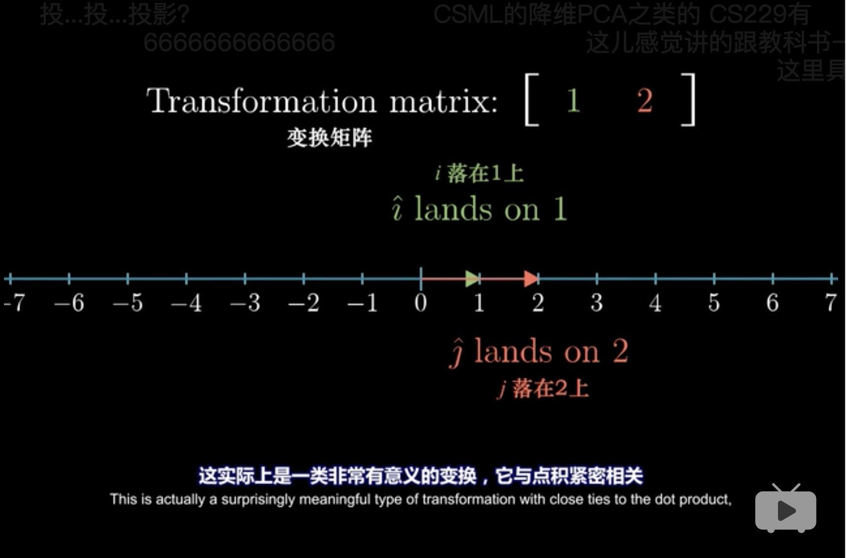
这种变换，也是靠线性变换完成的，假设 \(\begin{bmatrix}1&-2\end{bmatrix} \cdot \begin{bmatrix}4\\3\end{bmatrix}\)，可以认为\(\begin{bmatrix}1&-2\end{bmatrix}\)是变换矩阵可以认为\(\begin{bmatrix}4\\3\end{bmatrix}\)是向量。变换矩阵是拥有两个向量，但是都只有只有一维，因此完成了二维向一维的转换。这就叫做对偶性。

some_mtr <- 
    matrix(
        c(3,1)
        ,nrow = 2
    )
trans_mtr <- 
    matrix(
        c(-1,-2)
        ,nrow = 1
    )
some_mtr

##      [,1]
## [1,]    3
## [2,]    1

trans_mtr

##      [,1] [,2]
## [1,]   -1   -2

trans_mtr %*%  some_mtr #线性变换计算方式

##      [,1]
## [1,]   -5

(trans_mtr %>% c) %*% (some_mtr %>% c) # 点积计算方式

##      [,1]
## [1,]   -5

这只是一种计算方式，主要是为了给出几何形象的理解，不必深究。
\(v \cdot w\)和\(w \cdot v\)一样，顺序无关。这是点积的一个性质，不受到矩阵运算的严格意义影响。 (3Blue1Brown 2018, Edition 7)

7 叉积

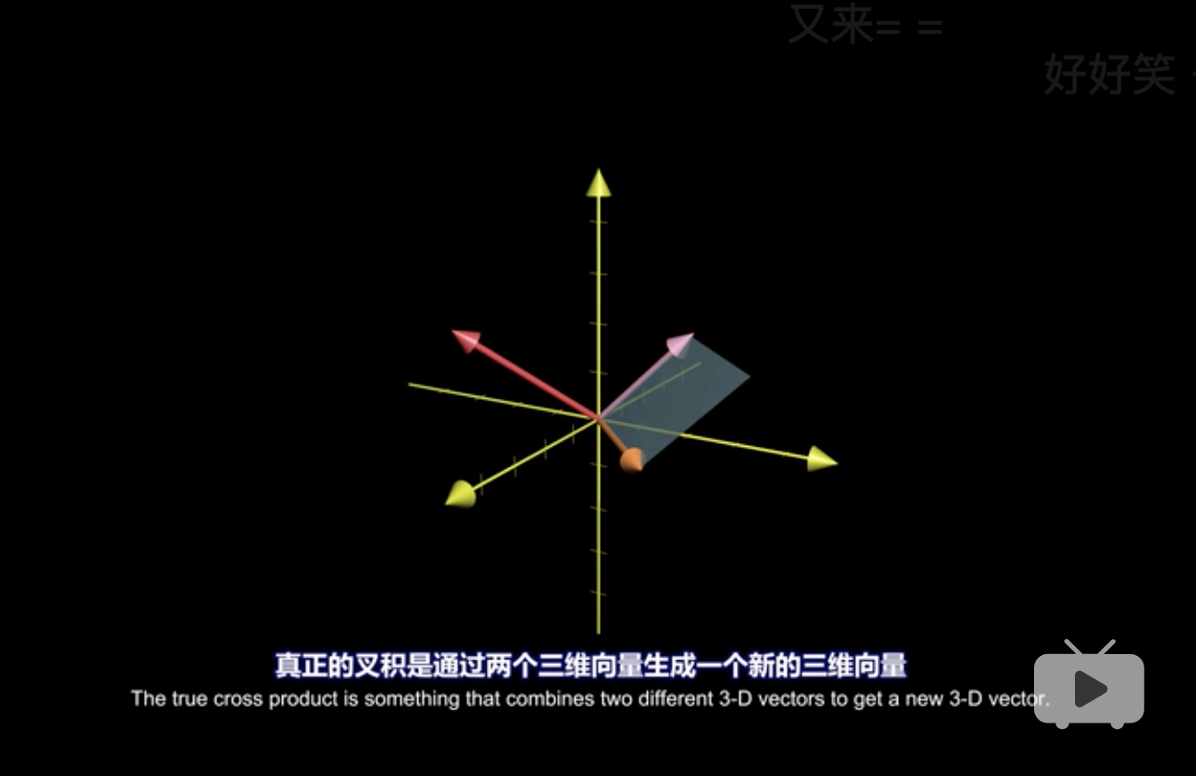
叉积产生后是一个向量。由浅入深，将叉积分为长度和方向两块解释。 (3Blue1Brown 2018, Edition 8.1,Edition 8.2)

首先定义叉积的长度，假设向量\(v\)和\(w\)，

\[v \times w = \det([v,w])\]

叉积就是det。直观理解，就是面积，见 3。当然因为方向不同，叉积可以为负¹。

叉积的方向上，有两种方式确定，

右手定则。
利用\(\det\)理解。在一个三维空间中，如果\(v \times w = \det([v,w])\)表示面积，那么\(u \times v \times w = \det([u,v,w])\)表示体积，在三维空间中表示平行六面体。其中\(u = \begin{bmatrix}x\\y\\z\end{bmatrix}\)。并且我们发现，这个体积关于\(u\)是线性的。 \[\det\begin{bmatrix}x&v_1&w_1\\y&v_2&w_2\\z&v_3&w_3\\\end{bmatrix}=x\det\begin{bmatrix}v_2&w_2\\v_3&w_3\\\end{bmatrix}+y\det\begin{bmatrix}v_1&w_1\\v_3&w_3\\\end{bmatrix}+z\det\begin{bmatrix}v_1&w_1\\v_2&w_2\\\end{bmatrix}\] 其中各个\(\det\)都是固定值，因此这是线性。因此可以利用对偶性，见 6，构建一个矩阵将\(u\)从三维降到一维，假设这个矩阵为\(p = [p_1,p_2,p_3]\)。因此满足， \[\begin{alignat}{2} [p_1,p_2,p_3]\begin{bmatrix}x\\y\\z\end{bmatrix} &= \det\begin{bmatrix}x&v_1&w_1\\y&v_2&w_2\\z&v_3&w_3\\\end{bmatrix} \\ x \cdot p_1 + y \cdot p_2 + z \cdot p_ 3 & = x\det\begin{bmatrix}v_2&w_2\\v_3&w_3\\\end{bmatrix}+ y\det\begin{bmatrix}v_1&w_1\\v_3&w_3\\\end{bmatrix}+ z\det\begin{bmatrix}v_1&w_1\\v_2&w_2\\\end{bmatrix} \\ \Rightarrow & \begin{cases} p_1 &= \det\begin{bmatrix}v_2&w_2\\v_3&w_3\\\end{bmatrix} \\ p_2 &= \det\begin{bmatrix}v_1&w_1\\v_3&w_3\\\end{bmatrix} \\ p_3 &= \det\begin{bmatrix}v_1&w_1\\v_2&w_2\\\end{bmatrix} \\ \end{cases} \\ \end{alignat}\] 并且根据点积的定义，见 6， \[\text{LHS} = p \cot u = |p| \cdot |u| \cdot \cos \theta\] 因此，LHS为\(u\)在\(p\)的投影\(|u| \cdot \cos \theta\)和\(p\)的乘积。因此紧接着推导的关键之处，体积处是向量\(v\)和\(w\)形成的面积乘以高，高是垂直于\(v\)和\(w\)形成的平面。点积处是\(u\)在\(p\)的投影\(|u| \cdot \cos \theta\)和\(p\)的乘积。因此向量\(p\)必须和高的方向一致，并且值为\(v\)和\(w\)形成的面积。那么只有\(p = v \times w\)。

8 基变换

基变换的内容主要设计三方面，假设有两个视角，A和B

A视角的向量在B视角中的表达
B视角的向量在A视角中的表达
A视角的变换矩阵在B视角中的表达

现在我们假设有两个不同的视角，我和 Jennifer。

在 Jennifer 的视角里面，有一个向量 \(\vec{v} = \begin{bmatrix}-1\\2\end{bmatrix}\)
在我的视角，这个向量表示为 \(\vec{v} = \begin{bmatrix}-4\\1\end{bmatrix}\)。
Jennifer 视角中的基\(\begin{bmatrix}1&0\\0&1\end{bmatrix}\)在我们的视角中为 \(i = \begin{bmatrix}2\\1\end{bmatrix}\) 和 \(j = \begin{bmatrix}-1\\1\end{bmatrix}\)

那么，这种视角的变换，只需要发生基变换可以完成(3Blue1Brown 2018, Edition 9)。以下是R代码的实现。

jennifer_mtr <- 
    matrix(
        c(-1,2)
        ,nrow = 2
    )
basic_vector_trans_mtr <- 
    matrix(
        c(
            c(2,1)
            ,c(-1,1)
        )
        ,nrow = 2
        ,byrow = F
    )
jennifer_mtr

##      [,1]
## [1,]   -1
## [2,]    2

basic_vector_trans_mtr

##      [,1] [,2]
## [1,]    2   -1
## [2,]    1    1

basic_vector_trans_mtr %*% jennifer_mtr

##      [,1]
## [1,]   -4
## [2,]    1

现在发生另外一种情况，

在我的视角里面，有一个向量 \(\vec{v} = \begin{bmatrix}3\\2\end{bmatrix}\)
1. 因为我们的是标准正交基，因此表示为 coordinates \((3,2)\)²。
在 Jennifer 的视角，这个向量表示为 \(\vec{v} = \begin{bmatrix}\frac{5}{3}\\\frac{1}{3}\end{bmatrix}\)。
Jennifer 视角中的基\(\begin{bmatrix}1&0\\0&1\end{bmatrix}\)在我们的视角中为 \(i = \begin{bmatrix}2\\1\end{bmatrix}\) 和 \(j = \begin{bmatrix}-1\\1\end{bmatrix}\)

me_mtr <- 
    matrix(
        c(3,2)
        ,nrow = 2
    )
basic_vector_trans_mtr <- 
    matrix(
        c(
            c(2,1)
            ,c(-1,1)
        )
        ,nrow = 2
        ,byrow = F
    )
me_mtr

##      [,1]
## [1,]    3
## [2,]    2

basic_vector_trans_mtr

##      [,1] [,2]
## [1,]    2   -1
## [2,]    1    1

solve(basic_vector_trans_mtr) %*% me_mtr

##           [,1]
## [1,] 1.6666667
## [2,] 0.3333333

现在发生另外一种情况，

在我的视角里面，发生了旋转变换，矩阵表示为 \(\vec{A} = \begin{bmatrix}0&-1\\1&0\end{bmatrix}\)
我们知道这种旋转变换在 Jennifer 的视角如何表达
Jennifer 视角中的基\(\begin{bmatrix}1&0\\0&1\end{bmatrix}\)在我们的视角中为 \(i = \begin{bmatrix}2\\1\end{bmatrix}\) 和 \(j = \begin{bmatrix}-1\\1\end{bmatrix}\)
便于理解的方式是在 Jennifer 的视角假设一个向量\(\vec{v} = \begin{bmatrix}-1\\2\end{bmatrix}\)，经过我的视角的旋转变换后，查看在 Jennifer 视角的表达。

jennifer_mtr <- 
    matrix(
        c(-1,2)
        ,nrow = 2
    )
basic_vector_trans_mtr <- 
    matrix(
        c(
            c(2,1)
            ,c(-1,1)
        )
        ,nrow = 2
        ,byrow = F
    )
rotation_mtr <- 
    matrix(
        c(
            c(0,1)
            ,c(-1,0)
        )
        ,nrow = 2
        ,byrow = F
    )
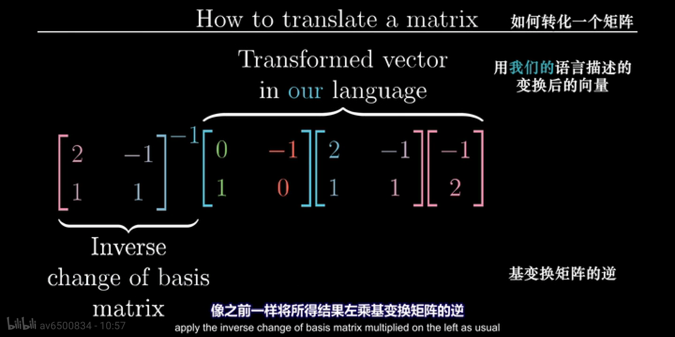
solve(basic_vector_trans_mtr) %*%
    rotation_mtr %*%
    basic_vector_trans_mtr %*% 
    jennifer_mtr

##           [,1]
## [1,] -1.666667
## [2,] -2.333333

注意这里的jennifer_mtr可以任意假设的，因此旋转变换在 Jennifer 的视角的表达为

solve(basic_vector_trans_mtr) %*%
    rotation_mtr %*%
    basic_vector_trans_mtr

##           [,1]       [,2]
## [1,] 0.3333333 -0.6666667
## [2,] 1.6666667 -0.3333333

9 特征向量和特征值

9.1 特征向量和特征值定义

The word “eigen” is German for “own”. (Eager 2018)

因此，特征向量和特征值强调的是一种“自我”不变的特性。

从几何角度，

假设有一个二维平面，现在进行线性变换，见 1，使用矩阵\(\vec{A}\)。
假如这个平面存在一个向量\(\vec{v}\)，在\(\vec{A}\)进行变换后，方向未发生变化 (180度变换也算未改变方向)，那么我们认为\(\vec{v}\)是\(\vec{A}\)这次变换的一个特征向量。
当然这个向量经过线性变换后，长度大小会发生改变，相乘一个标量\(\lambda\)，记作特征值。 (3Blue1Brown 2018, Edition 10)

An eigenvector is a scalar multiple of itself (“own”) when multiplied by A. (Eager 2018)

因此，当使用矩阵\(\vec{A}\)进行线性变换时，\(\vec{A}\)的特征向量\(\vec{v}\)只会进行使用标量进行变长变短，但是不会发生方向的改变。

用公式表示为

\[Av=\lambda v\]

其中\(v\)是特征向量， \(\lambda\)说、是特征值。

有一种特殊情况，在一个三维空间中，一个立方体，因为矩阵\(\vec{A}\)发生了旋转，那么旋转的轴就是特征向量。因为在这次变换中，旋转的轴没有发生方向变化，同时，\(\lambda=1\)。

9.2 跟空间压缩的关系

\[(A-\lambda I)v=0\]

更有意义的情况是，\(A-\lambda I\)变成了一个零向量。
因此，\(\det(A-\lambda I)=0\)，
假设\(A=\begin{bmatrix}a&b\\c&d\\\end{bmatrix}\)，因此\(A-\lambda I=\begin{bmatrix}a-\lambda&b\\c&d-\lambda\\\end{bmatrix}\)，
通过\(\lambda\)的变动，让\(\begin{bmatrix}b\\d\\\end{bmatrix}\)和 \(\begin{bmatrix}a\\c\\\end{bmatrix}\)这两个向量，靠拢，空间的压缩，最后实现重合。

9.3 \(\lambda\)的特殊情况

9.3.1 旋转矩阵

[数据与算法之美](https://mp.weixin.qq.com/s/eNzWRN0QxnJrD8la5YcfAw)

Figure 9.1: 数据与算法之美

旋转矩阵 rotation matrix \(\vec{A}\)是没有特征根的，平面因为\(\vec{A}\)旋转后，没有一个变量是不发生方向变换的。代数上，特征值和特征向量用复数表达。

例如，

rotation_mtr <- 
    matrix(
        c(0,1,-1,0)
        ,nrow = 2
        ,byrow = F
    )
rotation_mtr

##      [,1] [,2]
## [1,]    0   -1
## [2,]    1    0

eigen(rotation_mtr)

## eigen() decomposition
## $values
## [1] 0+1i 0-1i
## 
## $vectors
##                      [,1]                 [,2]
## [1,] 0.7071068+0.0000000i 0.7071068+0.0000000i
## [2,] 0.0000000-0.7071068i 0.0000000+0.7071068i

rotation_mtr - eigen(rotation_mtr)$values[1]*diag(2)

##      [,1]  [,2]
## [1,] 0-1i -1+0i
## [2,] 1+0i  0-1i

rotation_mtr - eigen(rotation_mtr)$values[2]*diag(2)

##      [,1]  [,2]
## [1,] 0+1i -1+0i
## [2,] 1+0i  0+1i

# 两个都是零向量

(rotation_mtr - eigen(rotation_mtr)$values[1]*diag(2)) %*% eigen(rotation_mtr)$vectors

##      [,1]               [,2]
## [1,] 0+0i 0.000000-1.414214i
## [2,] 0+0i 1.414214+0.000000i

(rotation_mtr - eigen(rotation_mtr)$values[2]*diag(2)) %*% eigen(rotation_mtr)$vectors

##                    [,1] [,2]
## [1,] 0.000000+1.414214i 0+0i
## [2,] 1.414214+0.000000i 0+0i

# 两个都是零向量

# {(rotation_mtr - eigen(rotation_mtr)$values[1]*diag(2)) %*% eigen(rotation_mtr)$vectors} %>% det
# {(rotation_mtr - eigen(rotation_mtr)$values[2]*diag(2)) %*% eigen(rotation_mtr)$vectors} %>% det
# 'determinant' not currently defined for complex matrices

代数上，

\[\begin{alignat}{2} (A-\lambda I)v&=0 \\ \det(A-\lambda I)&=0 \\ \begin{bmatrix} 0-\lambda&-1 \\ 1&0-\lambda \\ \end{bmatrix}&=0 \\ (-\lambda)^2-(-1)(1)&=0\\ \lambda^2+1=&0 \end{alignat}\]

9.3.2 剪切变换

剪切变换 shear matrix\(\vec{A}\)是只有唯一的特征根的，平面因为\(\vec{A}\)的一个向量发生旋转后，另一个向量保持原来的方向不变，因此这个向量就是特征向量，但是特征根是唯一的。

例如，

shear_mtr <- 
    matrix(
        c(1,1,0,1)
        ,nrow = 2
        ,byrow = T
    )
shear_mtr

##      [,1] [,2]
## [1,]    1    1
## [2,]    0    1

eigen(shear_mtr)

## eigen() decomposition
## $values
## [1] 1 1
## 
## $vectors
##      [,1]          [,2]
## [1,]    1 -1.000000e+00
## [2,]    0  2.220446e-16

shear_mtr - eigen(shear_mtr)$values[1]*diag(2)

##      [,1] [,2]
## [1,]    0    1
## [2,]    0    0

shear_mtr - eigen(shear_mtr)$values[2]*diag(2)

##      [,1] [,2]
## [1,]    0    1
## [2,]    0    0

# 两个都是零向量

(shear_mtr - eigen(shear_mtr)$values[1]*diag(2)) %*% eigen(shear_mtr)$vectors

##      [,1]         [,2]
## [1,]    0 2.220446e-16
## [2,]    0 0.000000e+00

(shear_mtr - eigen(shear_mtr)$values[2]*diag(2)) %*% eigen(shear_mtr)$vectors

##      [,1]         [,2]
## [1,]    0 2.220446e-16
## [2,]    0 0.000000e+00

# 两个都是零向量

{(shear_mtr - eigen(shear_mtr)$values[1]*diag(2)) %*% eigen(shear_mtr)$vectors} %>% det

## [1] 0

{(shear_mtr - eigen(shear_mtr)$values[2]*diag(2)) %*% eigen(shear_mtr)$vectors} %>% det

## [1] 0

# det = 0

\[\begin{alignat}{2} (A-\lambda I)v&=0 \\ \det(A-\lambda I)&=0 \\ \begin{bmatrix} 1-\lambda&1 \\ 0&1-\lambda \\ \end{bmatrix}&=0 \\ (1-\lambda)^2-&=0\\ \lambda&=1 \end{alignat}\]

9.3.3 一个特征值有多个特征向量

如果\(Av=\lambda v\)存在，那么\(A(2v)=\lambda (2v)\)存在，因此\(2v\)也是特征向量。

9.4 R实现

\[\begin{alignat}{2} (A-\lambda I)v&=0 \\ \end{alignat}\]

代码参考 Eager (2018 Chapter 3.10)。

A <- matrix(c(1,2,3,4),nrow = 2,byrow = 2)
A

##      [,1] [,2]
## [1,]    1    2
## [2,]    3    4

eigen(A)

## eigen() decomposition
## $values
## [1]  5.3722813 -0.3722813
## 
## $vectors
##            [,1]       [,2]
## [1,] -0.4159736 -0.8245648
## [2,] -0.9093767  0.5657675

A - eigen(A)$values[1]*diag(2)

##           [,1]      [,2]
## [1,] -4.372281  2.000000
## [2,]  3.000000 -1.372281

A - eigen(A)$values[2]*diag(2)

##          [,1]     [,2]
## [1,] 1.372281 2.000000
## [2,] 3.000000 4.372281

# 两个都是零向量


(A - eigen(A)$values[1]*diag(2)) %*% eigen(A)$vectors

##               [,1]      [,2]
## [1,] -2.220446e-16  4.736764
## [2,]  2.220446e-16 -3.250087

(A - eigen(A)$values[2]*diag(2)) %*% eigen(A)$vectors

##           [,1] [,2]
## [1,] -2.389586    0
## [2,] -5.223971    0

# 两个都是零向量

{(A - eigen(A)$values[1]*diag(2)) %*% eigen(A)$vectors} %>% det

## [1] -3.301088e-16

{(A - eigen(A)$values[2]*diag(2)) %*% eigen(A)$vectors} %>% det

## [1] 0

# 零向量 det = 0

附录

9.5 三维空间中的线性变换

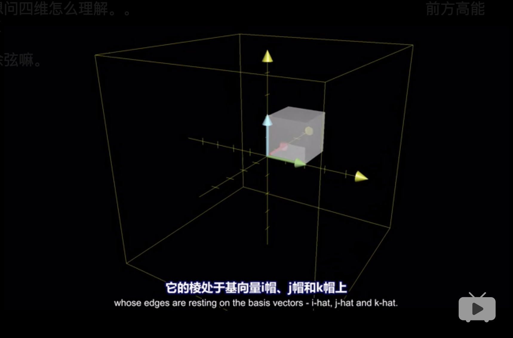
scale each basis vector. (3Blue1Brown 2018, 附注1)

与平面几何的理解类似，见 1。

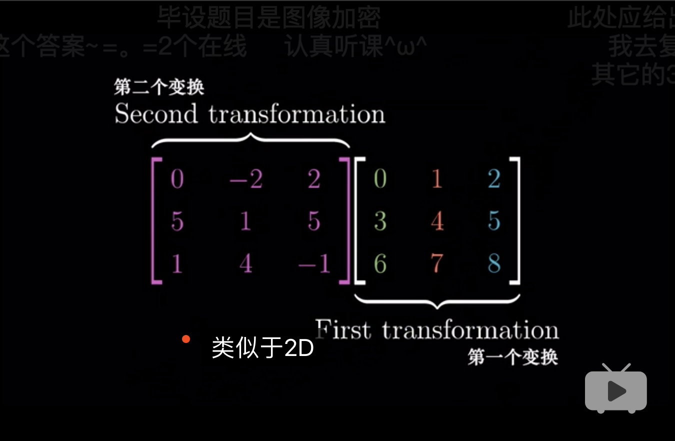
some_mtr <- 
    matrix(
        c(0,-2,2,5,1,5,1,4,-1)
        ,nrow = 3
        ,byrow = T
    )
basic_mtr <- 
    matrix(
        0:8
        ,nrow = 3
        ,byrow = T
    )
some_mtr

##      [,1] [,2] [,3]
## [1,]    0   -2    2
## [2,]    5    1    5
## [3,]    1    4   -1

basic_mtr

##      [,1] [,2] [,3]
## [1,]    0    1    2
## [2,]    3    4    5
## [3,]    6    7    8

some_mtr%*%diag(3)[,1]

##      [,1]
## [1,]    0
## [2,]    5
## [3,]    1

some_mtr%*%basic_mtr[,1]

##      [,1]
## [1,]    6
## [2,]   33
## [3,]    6

some_mtr%*%diag(3)[,2]

##      [,1]
## [1,]   -2
## [2,]    1
## [3,]    4

some_mtr%*%basic_mtr[,2]

##      [,1]
## [1,]    6
## [2,]   44
## [3,]   10

some_mtr%*%diag(3)[,3]

##      [,1]
## [1,]    2
## [2,]    5
## [3,]   -1

some_mtr%*%basic_mtr[,3]

##      [,1]
## [1,]    6
## [2,]   55
## [3,]   14

some_mtr%*%diag(3)

##      [,1] [,2] [,3]
## [1,]    0   -2    2
## [2,]    5    1    5
## [3,]    1    4   -1

some_mtr%*%basic_mtr

##      [,1] [,2] [,3]
## [1,]    6    6    6
## [2,]   33   44   55
## [3,]    6   10   14

9.6 非方阵

从几何上理解，有两种，

假设有一个向量，

some_mtr <- 
    matrix(
        c(3,1,4,1,5,9)
        ,nrow=3
        ,byrow = T
    )
some_mtr

##      [,1] [,2]
## [1,]    3    1
## [2,]    4    1
## [3,]    5    9

第一种非方阵表示，两列表示两个基，三行表示三维。在三维空间中，还是两个向量，虽然没有体积，但是是一个平面，因为只有两个基，还有一个被压缩到了原点，零向量。并且方向在三维空间中都有标志。 (3Blue1Brown 2018, 附注2)

被压缩到了原点的几何意义，见 5。

第二种非方阵表示，两列表示二维，三行表示三个基。

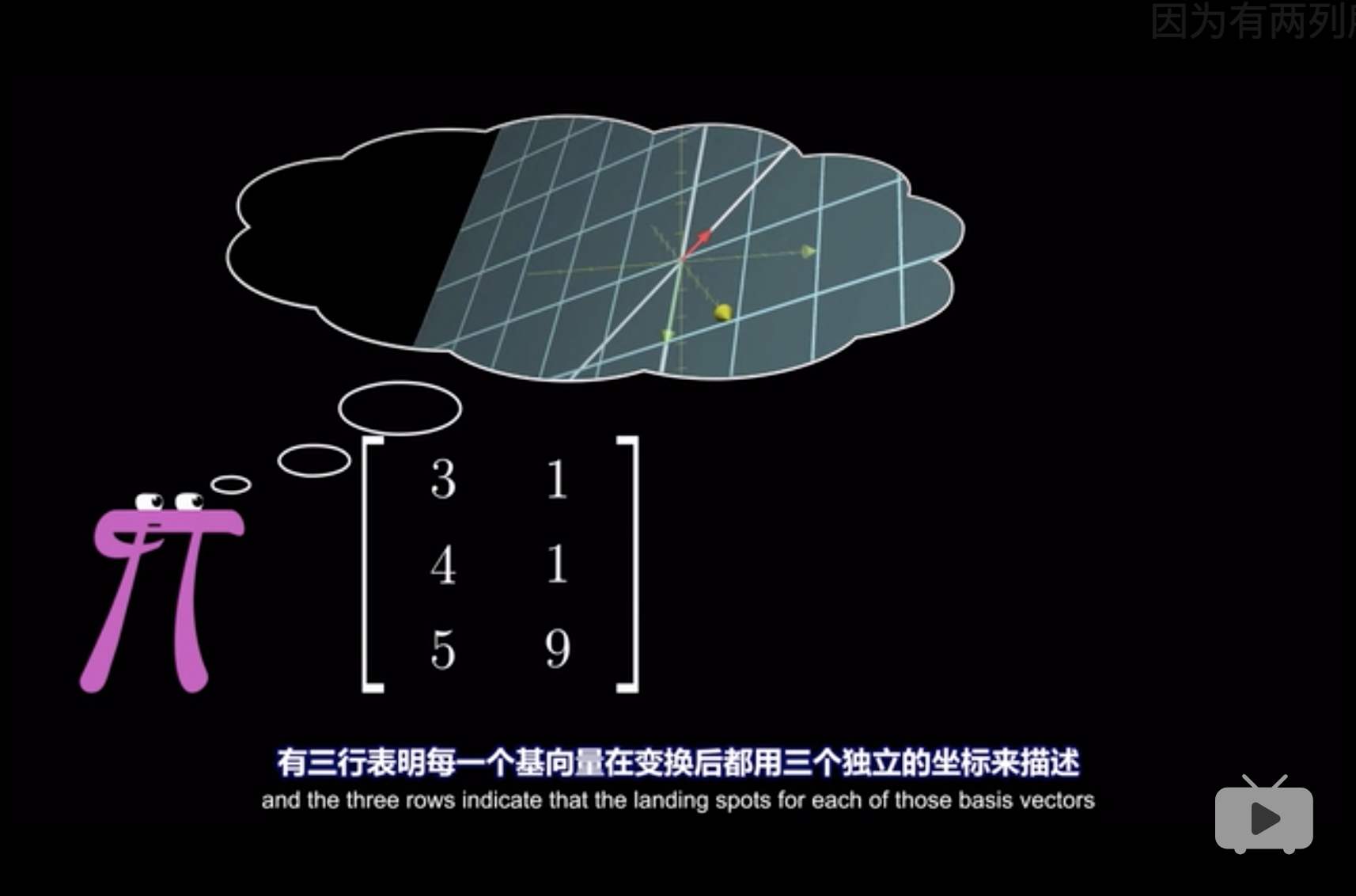
平面上有三个基，但是显然平面是只需要两个的。

同理，两维降到一维，有两个基，那么就是一条线上，两个向量，可同向或者反向。

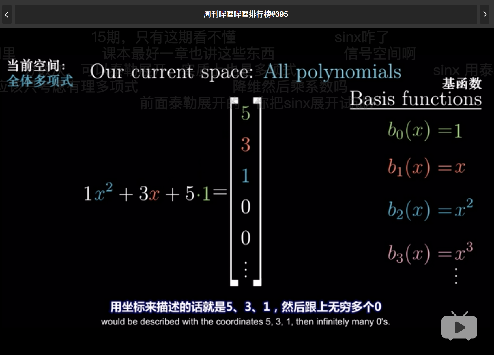
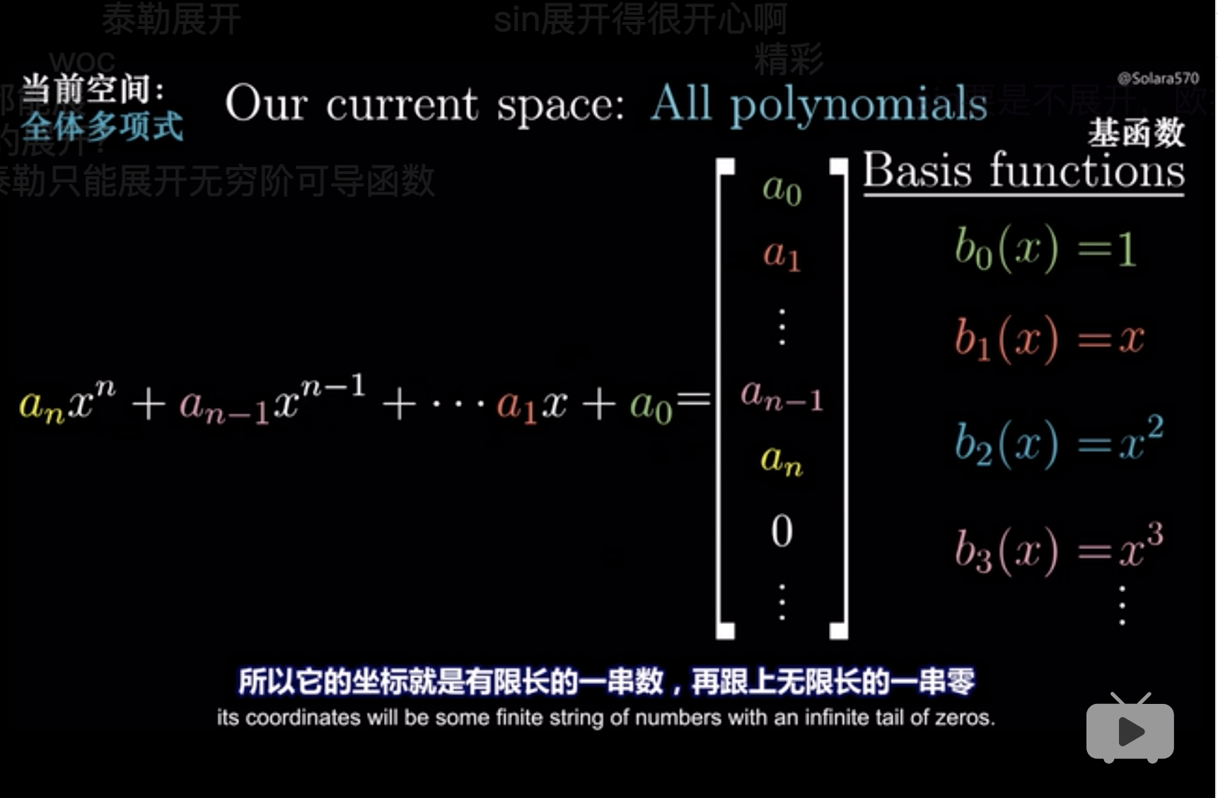
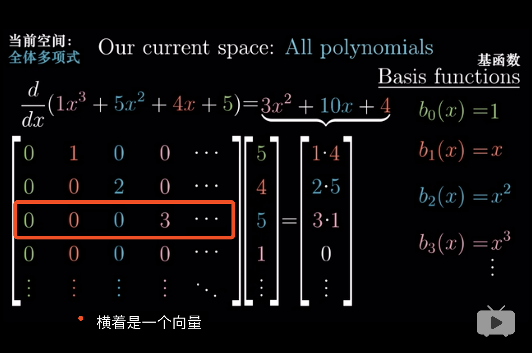
9.7 抽象、向量、函数

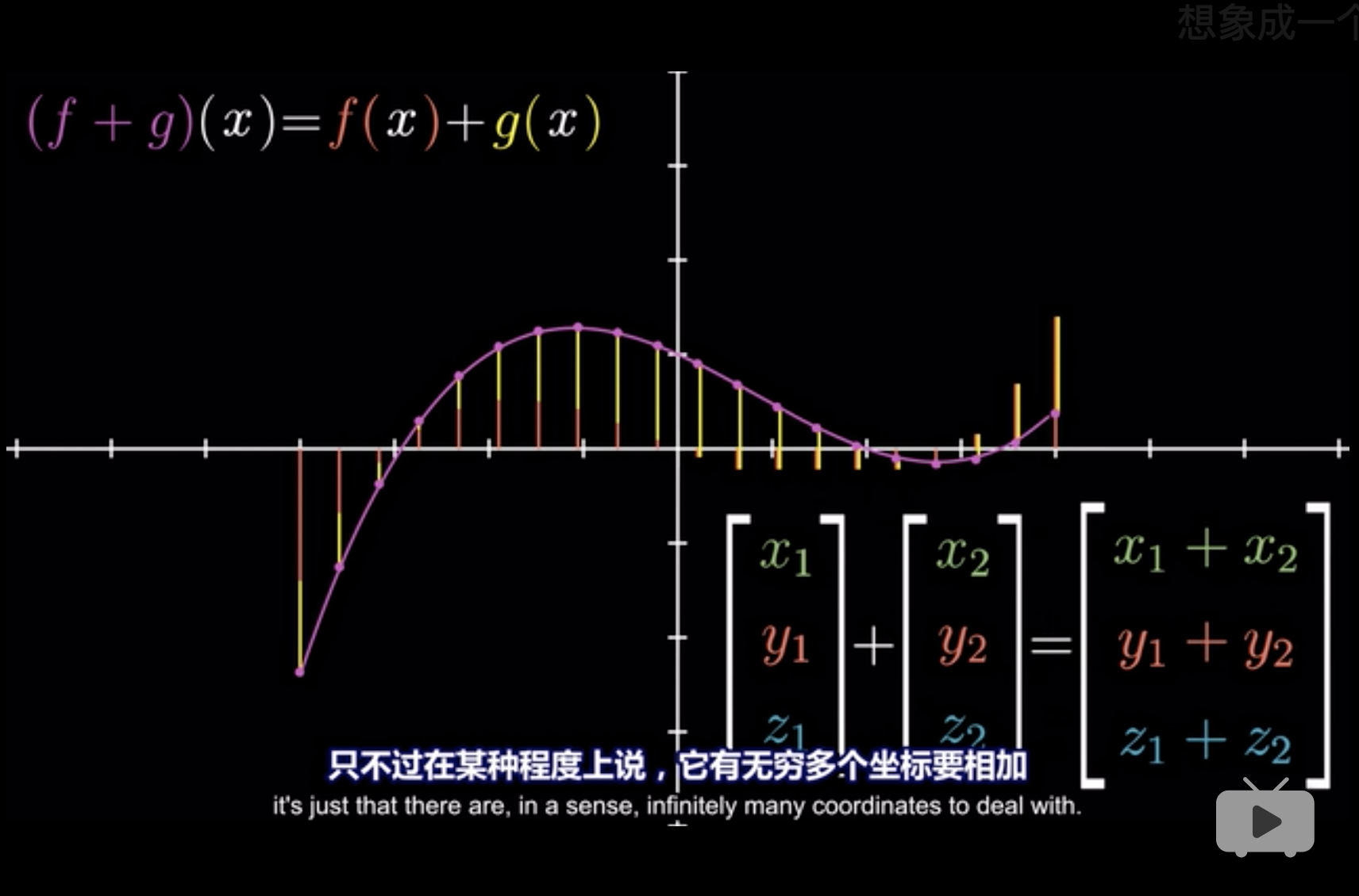
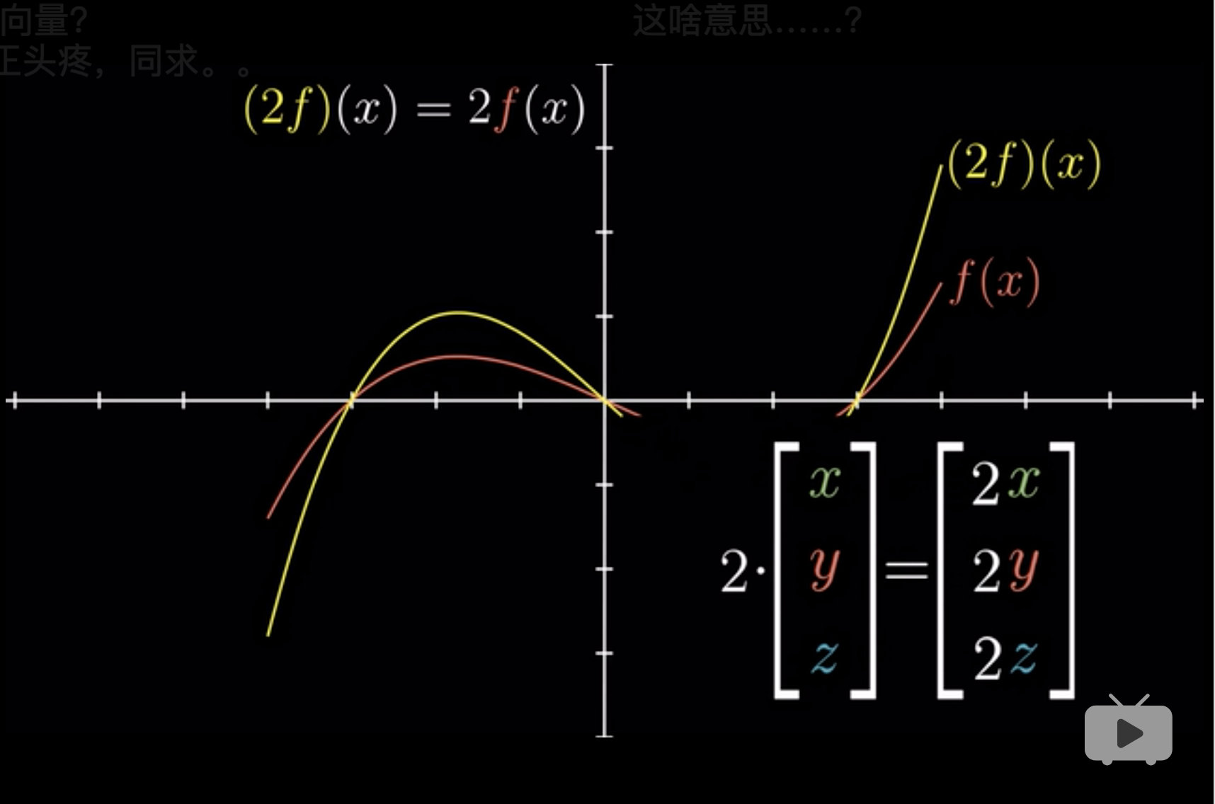
向量不仅仅是箭头和数字，它表示一切，满足可加性和放缩性的物质，就可以线性变换³。 (3Blue1Brown 2018, Edition 11)

可加性 (adding): \(f(x) +f(y) = f(x+y)\)
放缩性 (scaling): \(f(cx)=cf(x)\)

但是我们都知道，

Abstractness is the price of generality. (3Blue1Brown 2018, Edition 11)

抽象是普适的代价。因此，在理解线性代数时，用网格线、几何来理解，但是实际上，它不仅仅可用网格线，只要满足可加性和放缩性都可以适用。

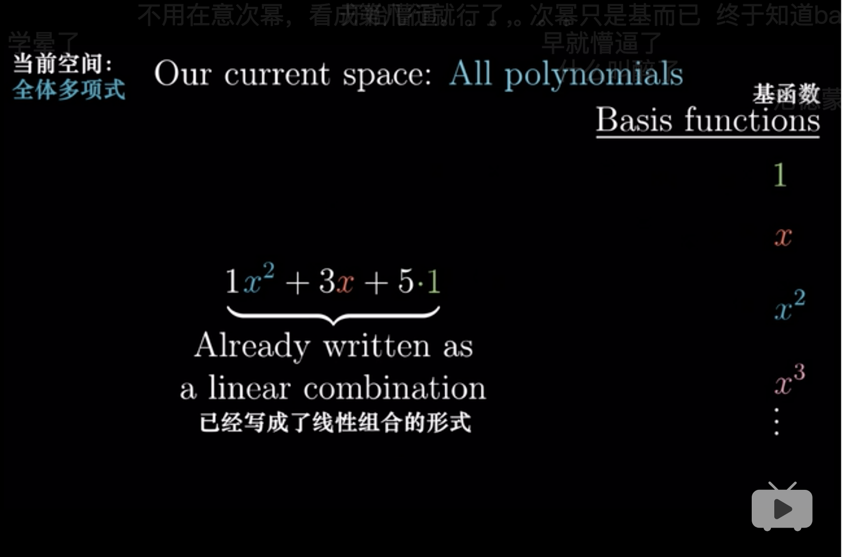
多项式表达
求导表达

9.8 Linear Algebra in R

9.8.1 元素计算

矩阵计算一般分两种

Element-wise operations 元素计算
Basic Matrix Operations 矩阵计算

source(here::here("R/sample_data.R"))
A

##      [,1] [,2] [,3] [,4] [,5]
## [1,]    1    2    3    4    5
## [2,]    6    7    8    9   10
## [3,]   11   12   13   14   15
## [4,]   16   17   18   19   20
## [5,]   21   22   23   24   25

##      [,1] [,2] [,3] [,4] [,5]
## [1,]   25   30   35   40   45
## [2,]   26   31   36   41   46
## [3,]   27   32   37   42   47
## [4,]   28   33   38   43   48
## [5,]   29   34   39   44   49

A / B

##           [,1]       [,2]       [,3]      [,4]      [,5]
## [1,] 0.0400000 0.06666667 0.08571429 0.1000000 0.1111111
## [2,] 0.2307692 0.22580645 0.22222222 0.2195122 0.2173913
## [3,] 0.4074074 0.37500000 0.35135135 0.3333333 0.3191489
## [4,] 0.5714286 0.51515152 0.47368421 0.4418605 0.4166667
## [5,] 0.7241379 0.64705882 0.58974359 0.5454545 0.5102041

A ^ B # 新颖

##              [,1]         [,2]         [,3]         [,4]         [,5]
## [1,] 1.000000e+00 1.073742e+09 5.003155e+16 1.208926e+24 2.842171e+31
## [2,] 1.705817e+20 1.577754e+26 3.245186e+32 1.330279e+39 1.000000e+46
## [3,] 1.310999e+28 3.418219e+34 1.644008e+41 1.372074e+48 1.889249e+55
## [4,] 5.192297e+33 4.025450e+40 5.015973e+47 9.691809e+54 2.814750e+62
## [5,] 2.209833e+38 4.389056e+45 1.280518e+53 5.361603e+60 3.155444e+68

9.8.2 矩阵合并

参考 Wang et al. (2019) ，如模型的特征时常是需要 concat 的。如

\[\boldsymbol{Y}=\sigma([\boldsymbol{X} \| \boldsymbol{G} \boldsymbol{X}] \boldsymbol{W})\]

表示 \(\boldsymbol{X}\) 和 \(\boldsymbol{G} \boldsymbol{X}\) 合并，\(\|\) 是连接符号。

source(here::here("R/sample_data.R"))
cbind(A, B)

##      [,1] [,2] [,3] [,4] [,5] [,6] [,7] [,8] [,9] [,10]
## [1,]    1    2    3    4    5   25   30   35   40    45
## [2,]    6    7    8    9   10   26   31   36   41    46
## [3,]   11   12   13   14   15   27   32   37   42    47
## [4,]   16   17   18   19   20   28   33   38   43    48
## [5,]   21   22   23   24   25   29   34   39   44    49

rbind(A, B)

##       [,1] [,2] [,3] [,4] [,5]
##  [1,]    1    2    3    4    5
##  [2,]    6    7    8    9   10
##  [3,]   11   12   13   14   15
##  [4,]   16   17   18   19   20
##  [5,]   21   22   23   24   25
##  [6,]   25   30   35   40   45
##  [7,]   26   31   36   41   46
##  [8,]   27   32   37   42   47
##  [9,]   28   33   38   43   48
## [10,]   29   34   39   44   49

9.8.3 Basic Calculation

x <- 1:7
y <- 2:8
z <- rep(1,3)
x

## [1] 1 2 3 4 5 6 7

## [1] 2 3 4 5 6 7 8

x * y

## [1]  2  6 12 20 30 42 56

x+z

## [1] 2 3 4 5 6 7 8

类似于data.frame里面的相乘。
longer object length is not a multiple of shorter object length说明，最后R自动修改了z为7的长度。

a <- matrix(1,3,2)
b <- matrix(-1,3,2)
a

##      [,1] [,2]
## [1,]    1    1
## [2,]    1    1
## [3,]    1    1

##      [,1] [,2]
## [1,]   -1   -1
## [2,]   -1   -1
## [3,]   -1   -1

a+b

##      [,1] [,2]
## [1,]    0    0
## [2,]    0    0
## [3,]    0    0

a %*% t(b)

##      [,1] [,2] [,3]
## [1,]   -2   -2   -2
## [2,]   -2   -2   -2
## [3,]   -2   -2   -2

a <- data.table(
    x = 1:2
    ,y = 3:4
)
a*a

a <- matrix(1:4,nrow = 2,byrow = TRUE)
a*a

##      [,1] [,2]
## [1,]    1    4
## [2,]    9   16

a%*%a

##      [,1] [,2]
## [1,]    7   10
## [2,]   15   22

I <- diag(2)
I

##      [,1] [,2]
## [1,]    1    0
## [2,]    0    1

I*I

##      [,1] [,2]
## [1,]    1    0
## [2,]    0    1

I%*%I

##      [,1] [,2]
## [1,]    1    0
## [2,]    0    1

9.8.4 Inverse Matrix

A <- matrix(c(1,2,-1,2),nrow = 2,byrow = T)

# Take the inverse of the 2 by 2 identity matrix
solve(diag(2))

##      [,1] [,2]
## [1,]    1    0
## [2,]    0    1

# Take the inverse of the matrix A
Ainv <- solve(A)

# Multiply A by its inverse on the left
Ainv%*%A

##      [,1] [,2]
## [1,]    1    0
## [2,]    0    1

# Multiply A by its inverse on the right
A%*%Ainv

##      [,1] [,2]
## [1,]    1    0
## [2,]    0    1

对于非方阵，见 9.6，MASS包可以处理。 (Eager 2018, Chapter 3.1)

library(purrr)
library(MASS)
a <- matrix(c(2,3,-1,4,1,7),nrow = 3,byrow = T)
a

##      [,1] [,2]
## [1,]    2    3
## [2,]   -1    4
## [3,]    1    7

# solve(a)
# Error in solve.default(x) : 'a' (3 x 2) must be square
ginv(a)

##           [,1]        [,2]       [,3]
## [1,] 0.3333333 -0.30303030 0.03030303
## [2,] 0.0000000  0.09090909 0.09090909

ginv(a)%*%a

##      [,1]          [,2]
## [1,]    1 -1.110223e-16
## [2,]    0  1.000000e+00

# ？
# Find the rating vector the conventional way
r <- solve(M_mtr)%*%f_mtr
colnames(r) <- "Rating"
print(r)

# Find the rating vector using ginv
r <- ginv(M_mtr)%*%f_mtr
colnames(r) <- "Rating"
print(r)

9.8.5 matrix manipulation

M <- diag(12)
M[M==0] <- -1
# Add a row of 1's
M <- rbind(M, rep(1, 12))

# Add a column of -1's 
M <- cbind(M, rep(-1, 13))

# Change the element in the lower-right corner of the matrix M
M[13, 13] <- 1

# Print M
print(M)

##       [,1] [,2] [,3] [,4] [,5] [,6] [,7] [,8] [,9] [,10] [,11] [,12] [,13]
##  [1,]    1   -1   -1   -1   -1   -1   -1   -1   -1    -1    -1    -1    -1
##  [2,]   -1    1   -1   -1   -1   -1   -1   -1   -1    -1    -1    -1    -1
##  [3,]   -1   -1    1   -1   -1   -1   -1   -1   -1    -1    -1    -1    -1
##  [4,]   -1   -1   -1    1   -1   -1   -1   -1   -1    -1    -1    -1    -1
##  [5,]   -1   -1   -1   -1    1   -1   -1   -1   -1    -1    -1    -1    -1
##  [6,]   -1   -1   -1   -1   -1    1   -1   -1   -1    -1    -1    -1    -1
##  [7,]   -1   -1   -1   -1   -1   -1    1   -1   -1    -1    -1    -1    -1
##  [8,]   -1   -1   -1   -1   -1   -1   -1    1   -1    -1    -1    -1    -1
##  [9,]   -1   -1   -1   -1   -1   -1   -1   -1    1    -1    -1    -1    -1
## [10,]   -1   -1   -1   -1   -1   -1   -1   -1   -1     1    -1    -1    -1
## [11,]   -1   -1   -1   -1   -1   -1   -1   -1   -1    -1     1    -1    -1
## [12,]   -1   -1   -1   -1   -1   -1   -1   -1   -1    -1    -1     1    -1
## [13,]    1    1    1    1    1    1    1    1    1     1     1     1     1

solve(M) %>% 
    round(3)

##       [,1] [,2] [,3] [,4] [,5] [,6] [,7] [,8] [,9] [,10] [,11] [,12] [,13]
##  [1,]  0.5  0.0  0.0  0.0  0.0  0.0  0.0  0.0  0.0   0.0   0.0   0.0   0.5
##  [2,]  0.0  0.5  0.0  0.0  0.0  0.0  0.0  0.0  0.0   0.0   0.0   0.0   0.5
##  [3,]  0.0  0.0  0.5  0.0  0.0  0.0  0.0  0.0  0.0   0.0   0.0   0.0   0.5
##  [4,]  0.0  0.0  0.0  0.5  0.0  0.0  0.0  0.0  0.0   0.0   0.0   0.0   0.5
##  [5,]  0.0  0.0  0.0  0.0  0.5  0.0  0.0  0.0  0.0   0.0   0.0   0.0   0.5
##  [6,]  0.0  0.0  0.0  0.0  0.0  0.5  0.0  0.0  0.0   0.0   0.0   0.0   0.5
##  [7,]  0.0  0.0  0.0  0.0  0.0  0.0  0.5  0.0  0.0   0.0   0.0   0.0   0.5
##  [8,]  0.0  0.0  0.0  0.0  0.0  0.0  0.0  0.5  0.0   0.0   0.0   0.0   0.5
##  [9,]  0.0  0.0  0.0  0.0  0.0  0.0  0.0  0.0  0.5   0.0   0.0   0.0   0.5
## [10,]  0.0  0.0  0.0  0.0  0.0  0.0  0.0  0.0  0.0   0.5   0.0   0.0   0.5
## [11,]  0.0  0.0  0.0  0.0  0.0  0.0  0.0  0.0  0.0   0.0   0.5   0.0   0.5
## [12,]  0.0  0.0  0.0  0.0  0.0  0.0  0.0  0.0  0.0   0.0   0.0   0.5   0.5
## [13,] -0.5 -0.5 -0.5 -0.5 -0.5 -0.5 -0.5 -0.5 -0.5  -0.5  -0.5  -0.5  -5.0

\[M \times \text{rating} = f\]

M <- fread('../../picbackup/WNBA_Data_2017_M.csv')
f <- fread('../../picbackup/WNBA_Data_2017_f.csv')

M_mtr <- M %>% as.matrix # has column name
f_mtr <- f %>% as.matrix # has column name
solve(M_mtr)%*%f_mtr # with M's column name and f's column name

##              Differential
## Atlanta     -4.012938e+00
## Chicago     -5.156260e+00
## Connecticut  4.309525e+00
## Dallas      -2.608129e+00
## Indiana     -8.532958e+00
## Los Angeles  7.850327e+00
## Minnesota    1.061241e+01
## New York     2.541565e+00
## Phoenix      8.979110e-01
## San Antonio -6.181574e+00
## Seattle     -2.666953e-01
## Washington   5.468121e-01
## WNBA         1.043610e-14

9.8.6 Eigen*

主要使用函数eigen(Eager 2018, Chapter 3.6)

A <- matrix(c(-1,2,4,0,7,12,0,0,-4),nrow = 3,byrow = T)
A

##      [,1] [,2] [,3]
## [1,]   -1    2    4
## [2,]    0    7   12
## [3,]    0    0   -4

Eigen_mtr <- 
    matrix(
        c(
            c(0.2425356, 0.9701425, 0)
            ,c(-0.3789810, -0.6821657, 0.6253186)
            ,c(1,0,0)
        )
        ,nrow = 3
        ,byrow = T
    )
Eigen_mtr

##            [,1]       [,2]      [,3]
## [1,]  0.2425356  0.9701425 0.0000000
## [2,] -0.3789810 -0.6821657 0.6253186
## [3,]  1.0000000  0.0000000 0.0000000

# Show that 7 is an eigenvalue for A
A%*%c(0.2425356, 0.9701425, 0) - 7*c(0.2425356, 0.9701425, 0)

##       [,1]
## [1,] 2e-07
## [2,] 0e+00
## [3,] 0e+00

# Show that -4 is an eigenvalue for A
A%*%c(-0.3789810, -0.6821657, 0.6253186) - (-4)*c(-0.3789810, -0.6821657, 0.6253186)

##               [,1]
## [1,] -2.220446e-16
## [2,]  5.000000e-07
## [3,]  0.000000e+00

# Show that -1 is an eigenvalue for A
A%*%c(1,0,0) - (-1)*c(1,0,0)

##      [,1]
## [1,]    0
## [2,]    0
## [3,]    0

For the first eigenpair in the previous problem, show that double and half of the eigenvector used is still an eigenvector for the given eigenvalue. (Eager 2018, Chapter 3)

# Show that double an eigenvector is still an eigenvector
A%*%((2)*c(0.2425356, 0.9701425, 0)) - 7*(2)*c(0.2425356, 0.9701425, 0)

##       [,1]
## [1,] 4e-07
## [2,] 0e+00
## [3,] 0e+00

# Show half of an eigenvector is still an eigenvector
A%*%((0.5)*c(0.2425356, 0.9701425, 0)) - 7*(0.5)*c(0.2425356, 0.9701425, 0)

##       [,1]
## [1,] 1e-07
## [2,] 0e+00
## [3,] 0e+00

Show that, for each eigenvalue lambda (λ), that the determinant of \(\lambda I - A\) is equal to zero. (Eager 2018)

A <- matrix(c(1,2,1,1),nrow = 2,byrow = 2)

# Compute the eigenvalues of A and store in Lambda
Lambda <- eigen(A)

# Print eigenvalues
print(Lambda$values[1])

## [1] 2.414214

print(Lambda$values[2])

## [1] -0.4142136

# Verify that these numbers satisfy the conditions of being an eigenvalue
det(Lambda$values[1]*diag(2) - A)

## [1] -3.140185e-16

det(Lambda$values[2]*diag(2) - A)

## [1] -3.140185e-16

\[A \cdot v = \lambda \cdot v\]

# Find the eigenvectors of A and store them in Lambda
Lambda <- eigen(A)

# Print eigenvectors
print(Lambda$vectors[, 1])

## [1] 0.8164966 0.5773503

print(Lambda$vectors[, 2])

## [1] -0.8164966  0.5773503

# Verify that these eigenvectors & their associated eigenvalues satisfy Av - lambda v = 0
Lambda$values[1]*Lambda$vectors[, 1] - A%*%Lambda$vectors[, 1]

##      [,1]
## [1,]    0
## [2,]    0

Lambda$values[2]*Lambda$vectors[, 2] - A%*%Lambda$vectors[, 2]

##               [,1]
## [1,] -1.110223e-16
## [2,]  8.326673e-17

9.8.7 Cases in Markov Models

M是 Markov matrix (Eager 2018, Chapter 3.14)

M <- matrix(
    c(
        c(0.980, 0.005, 0.005, 0.010)
        ,c(0.005, 0.980, 0.010, 0.005)
        ,c(0.005, 0.010, 0.980, 0.005)
        ,c(0.010, 0.005, 0.005, 0.980)
    )
    ,nrow = 4
    ,byrow = T
)

M_0 <- M
M_0

##       [,1]  [,2]  [,3]  [,4]
## [1,] 0.980 0.005 0.005 0.010
## [2,] 0.005 0.980 0.010 0.005
## [3,] 0.005 0.010 0.980 0.005
## [4,] 0.010 0.005 0.005 0.980

for (j in 1:999) {M_0 <- M%*%M_0}
M_0

##      [,1] [,2] [,3] [,4]
## [1,] 0.25 0.25 0.25 0.25
## [2,] 0.25 0.25 0.25 0.25
## [3,] 0.25 0.25 0.25 0.25
## [4,] 0.25 0.25 0.25 0.25

M_0 %*% M_0

##      [,1] [,2] [,3] [,4]
## [1,] 0.25 0.25 0.25 0.25
## [2,] 0.25 0.25 0.25 0.25
## [3,] 0.25 0.25 0.25 0.25
## [4,] 0.25 0.25 0.25 0.25

可以发现矩阵进行>1000次后，所有元素变成0.25

# This code iterates mutation 100 times
x <- c(1, 0, 0, 0)
for (j in 1:1000) {x <- M%*%x}

# Print x
x

##      [,1]
## [1,] 0.25
## [2,] 0.25
## [3,] 0.25
## [4,] 0.25

M_0 %*% x

##      [,1]
## [1,] 0.25
## [2,] 0.25
## [3,] 0.25
## [4,] 0.25

# Print and scale the first eigenvector of M
Lambda <- eigen(M)
v1 <- Lambda$vectors[, 1]/sum(Lambda$vectors[, 1])

print(v1)

## [1] 0.25 0.25 0.25 0.25

9.8.8 Cases in PCA

combine <- fread('../../picbackup/DataCampCombine.csv')

# Extract columns 5-12 of combine
A <- combine[, 5:12]

# Make A into a matrix
A <- as.matrix(A)

# Subtract the mean of all columns
A[, 1] <- A[, 1] - mean(A[, 1])
A[, 2] <- A[, 2] - mean(A[, 2])
A[, 3] <- A[, 3] - mean(A[, 3])
A[, 4] <- A[, 4] - mean(A[, 4])
A[, 5] <- A[, 5] - mean(A[, 5])
A[, 6] <- A[, 6] - mean(A[, 6])
A[, 7] <- A[, 7] - mean(A[, 7])
A[, 8] <- A[, 8] - mean(A[, 8])
A %>% head

##            height     weight       forty  vertical     bench  broad_jump
## [1,] -2.992720971 -60.087348 -0.43158406  2.401733 -7.091854  13.8097054
## [2,] -0.992720971  45.912652  0.52841594 -6.098267  5.908146 -14.1902946
## [3,]  3.007279029   3.912652 -0.14158406 -1.598267 -4.091854  -0.1902946
## [4,]  0.007279029 -54.087348 -0.47158406  8.401733 -5.091854  17.8097054
## [5,]  2.007279029   4.912652  0.05841594 -2.598267 -1.091854   4.8097054
## [6,]  4.007279029   9.912652 -0.21158406  5.901733 -3.091854  14.8097054
##       three_cone     shuttle
## [1,] -0.59571924 -0.42854766
## [2,]  0.50428076  0.30145234
## [3,]  0.03428076 -0.02854766
## [4,] -0.74571924 -0.37854766
## [5,] -0.18571924 -0.17854766
## [6,]  0.22428076  0.07145234

\[\frac{A^TA}{n-1}\]

# Create matrix B from equation in instructions
B <- t(A)%*%A/(nrow(A) - 1)
B

##                 height      weight       forty    vertical       bench
## height       7.1597944   90.788084  0.52676257   -5.065512   6.2780614
## weight      90.7880840 2105.176834 13.04832553 -132.887401 188.5644427
## forty        0.5267626   13.048326  0.10318906   -1.034265   0.9549273
## vertical    -5.0655119 -132.887401 -1.03426459   18.232972  -8.7243553
## bench        6.2780614  188.564443  0.95492726   -8.724355  40.8989801
## broad_jump -11.2472274 -330.417460 -2.55786742   33.083582 -24.1124924
## three_cone   0.5955444   15.944407  0.11523591   -1.245058   1.2152061
## shuttle      0.3912377    9.644035  0.06894544   -0.811669   0.6913887
##             broad_jump  three_cone     shuttle
## height      -11.247227  0.59554442  0.39123769
## weight     -330.417460 15.94440664  9.64403467
## forty        -2.557867  0.11523591  0.06894544
## vertical     33.083582 -1.24505770 -0.81166895
## bench       -24.112492  1.21520610  0.69138865
## broad_jump   90.079934 -3.11504850 -1.89762575
## three_cone   -3.115048  0.18612283  0.09866407
## shuttle      -1.897626  0.09866407  0.07283010

# Compare 1st element of B to 1st column of variance of A
B[1,1]

## [1] 7.159794

var(A[, 1])

## [1] 7.159794

# Compare 1st element of 2nd column and row element of B to 1st and 2nd columns of A 
B[1, 2]

## [1] 90.78808

B[2, 1]

## [1] 90.78808

cov(A[, 1], A[, 2])

## [1] 90.78808

PCA的理解，相关性越高，越冗余(redundant)。 (Eager 2018, Chapter 4.3) 这也是求解Cov的一个原因即发现这种Redundancy。

# Find eigenvalues of B
V <- eigen(B)

# Print eigenvalues
V$values

## [1] 2.187628e+03 4.403246e+01 2.219205e+01 5.267129e+00 2.699702e+00
## [6] 6.317016e-02 1.480866e-02 1.307283e-02

library(formattable)
V$values %>% 
  as_tibble() %>% 
  mutate(value/sum(value) %>% percent())

The profile of the data can be attributed to one linear combination of the data. (Eager 2018, Chapter 4)

~~The profile of the data~~ \(\to\) the variance of data.

9.8.9 Completed

9.9 diag 函数用法

在 R 中，diag 的反函数是其本身。

a <- 1:3
(a_matrix <- diag(a))

##      [,1] [,2] [,3]
## [1,]    1    0    0
## [2,]    0    2    0
## [3,]    0    0    3

diag(a_matrix)

## [1] 1 2 3

diag(5)

##      [,1] [,2] [,3] [,4] [,5]
## [1,]    1    0    0    0    0
## [2,]    0    1    0    0    0
## [3,]    0    0    1    0    0
## [4,]    0    0    0    1    0
## [5,]    0    0    0    0    1

参考文献

3Blue1Brown. 2018. “线性代数的本质.” 2018. https://www.bilibili.com/video/av16144388/.

Eager, Eric. 2018. “Linear Algebra for Data Science in R.” DataCamp. 2018. https://www.datacamp.com/courses/linear-algebra-for-data-science-in-r.

Wang, Zhongdao, Liang Zheng, Yali Li, and Shengjin Wang. 2019. “Linkage Based Face Clustering via Graph Convolution Network.”

1. 如果方向反了，例如 \(w \times v = \det(\begin{bmatrix}w_1&v_1\\w_2&v_2\\w_3&v_3\\\end{bmatrix})\)。那么，\(\det<0\) 因为线性变换，相当于平面180度变化。因此面积表示为负。
2. 并且\(v\)和\(w\)越垂直，\(v \times w\)绝对值越大。反之越小。
↩︎
coordinates这个词要加s，一直忘记。 scalar 就是标量的意思，一直在用。↩︎
一共有8中公理。

↩︎

线性代数学习笔记

线性代数学习笔记

1 线性变换几何理解

2 矩阵乘法理解

3 用面积理解行列式

3.1 det < 0 的情况

3.2 如何理解反转

3.3 det 的计算公式推导

4 逆矩阵

4.1 det(A) = 0

4.2 \(\det(A^{-1}A)=1\)

5 列空间、秩与零空间

6 点积

7 叉积

8 基变换

9 特征向量和特征值

9.1 特征向量和特征值定义

9.2 跟空间压缩的关系

9.3 \(\lambda\)的特殊情况

9.3.1 旋转矩阵

9.3.2 剪切变换

9.3.3 一个特征值有多个特征向量

9.4 R实现

附录

9.5 三维空间中的线性变换

9.6 非方阵

9.7 抽象、向量、函数

9.8 Linear Algebra in R

9.8.1 元素计算

9.8.2 矩阵合并

9.8.3 Basic Calculation

9.8.4 Inverse Matrix

9.8.5 matrix manipulation

9.8.6 Eigen*

9.8.7 Cases in Markov Models

9.8.8 Cases in PCA

9.8.9 Completed

9.9 diag 函数用法

参考文献

线性代数 学习笔记

1 线性变换几何理解

2 矩阵乘法理解

3 用面积理解行列式

3.1 det < 0 的情况

3.2 如何理解反转

3.3 det 的计算公式推导

4 逆矩阵

4.1 det(A) = 0

4.2 \(\det(A^{-1}A)=1\)

5 列空间、秩与零空间

6 点积

7 叉积

8 基变换

9 特征向量和特征值

9.1 特征向量和特征值定义

9.2 跟空间压缩的关系

9.3 \(\lambda\)的特殊情况

9.3.1 旋转矩阵

9.3.2 剪切变换

9.3.3 一个特征值有多个特征向量

9.4 R实现

附录

9.5 三维空间中的线性变换

9.6 非方阵

9.7 抽象、向量、函数

9.8 Linear Algebra in R

9.8.1 元素计算

9.8.2 矩阵合并

9.8.3 Basic Calculation

9.8.4 Inverse Matrix

9.8.5 matrix manipulation

9.8.6 Eigen*

9.8.7 Cases in Markov Models

9.8.8 Cases in PCA

9.8.9 Completed

9.9 diag 函数用法

参考文献

线性代数学习笔记