R 数据清洗学习笔记
2019-05-05
- 使用 RMarkdown 的
child参数,进行文档拼接。 - 这样拼接以后的笔记方便复习。
- 相关问题提交到 GitHub
1 清洗数据的配置
参考 Carchedi (2016a)
其实数据科学,就这四个步骤,不要想太复杂。 但是 cleaning 这个过程一般需要 75% 以上的时间。
2 简单EDA
参考 Carchedi (2016a)
No one likes missing data, but it is dangerous to assume that it can simply be removed or replaced. Sometimes missing data tells us something important about whatever it is that we’re measuring (i.e. the value of the variable that is missing may be related to - the reason it is missing). Such data is called Missing not at Random, or MNAR. DataCamp
因此变量的空值不要随便覆盖,这是数据清理工作中需要注意的。
library(readr)
weather <- read_rds("datasets/weather.rds")

# View the first 6 rows of data
head(weather)
# View the last 6 rows of data
tail(weather)# View a condensed summary of the data
str(weather)## 'data.frame': 286 obs. of 35 variables:
## $ X : int 1 2 3 4 5 6 7 8 9 10 ...
## $ year : int 2014 2014 2014 2014 2014 2014 2014 2014 2014 2014 ...
## $ month : int 12 12 12 12 12 12 12 12 12 12 ...
## $ measure: chr "Max.TemperatureF" "Mean.TemperatureF" "Min.TemperatureF" "Max.Dew.PointF" ...
## $ X1 : chr "64" "52" "39" "46" ...
## $ X2 : chr "42" "38" "33" "40" ...
## $ X3 : chr "51" "44" "37" "49" ...
## $ X4 : chr "43" "37" "30" "24" ...
## $ X5 : chr "42" "34" "26" "37" ...
## $ X6 : chr "45" "42" "38" "45" ...
## $ X7 : chr "38" "30" "21" "36" ...
## $ X8 : chr "29" "24" "18" "28" ...
## $ X9 : chr "49" "39" "29" "49" ...
## $ X10 : chr "48" "43" "38" "45" ...
## $ X11 : chr "39" "36" "32" "37" ...
## $ X12 : chr "39" "35" "31" "28" ...
## $ X13 : chr "42" "37" "32" "28" ...
## $ X14 : chr "45" "39" "33" "29" ...
## $ X15 : chr "42" "37" "32" "33" ...
## $ X16 : chr "44" "40" "35" "42" ...
## $ X17 : chr "49" "45" "41" "46" ...
## $ X18 : chr "44" "40" "36" "34" ...
## $ X19 : chr "37" "33" "29" "25" ...
## $ X20 : chr "36" "32" "27" "30" ...
## $ X21 : chr "36" "33" "30" "30" ...
## $ X22 : chr "44" "39" "33" "39" ...
## $ X23 : chr "47" "45" "42" "45" ...
## $ X24 : chr "46" "44" "41" "46" ...
## $ X25 : chr "59" "52" "44" "58" ...
## $ X26 : chr "50" "44" "37" "31" ...
## $ X27 : chr "52" "45" "38" "34" ...
## $ X28 : chr "52" "46" "40" "42" ...
## $ X29 : chr "41" "36" "30" "26" ...
## $ X30 : chr "30" "26" "22" "10" ...
## $ X31 : chr "30" "25" "20" "8" ...因此这个数据集的质量可以用DataExplorer包来检验。
bmi <- read_csv("datasets/bmi_clean.csv")

# Load dplyr
library(dplyr)

# Check the structure of bmi, the dplyr way
glimpse(bmi)
## Observations: 199
## Variables: 30
## $ Country <chr> "Afghanistan", "Albania", "Algeria", "Andorra", "Angol...
## $ Y1980 <dbl> 21.48678, 25.22533, 22.25703, 25.66652, 20.94876, 23.3...
## $ Y1981 <dbl> 21.46552, 25.23981, 22.34745, 25.70868, 20.94371, 23.3...
## $ Y1982 <dbl> 21.45145, 25.25636, 22.43647, 25.74681, 20.93754, 23.4...
## $ Y1983 <dbl> 21.43822, 25.27176, 22.52105, 25.78250, 20.93187, 23.5...
## $ Y1984 <dbl> 21.42734, 25.27901, 22.60633, 25.81874, 20.93569, 23.6...
## $ Y1985 <dbl> 21.41222, 25.28669, 22.69501, 25.85236, 20.94857, 23.7...
## $ Y1986 <dbl> 21.40132, 25.29451, 22.76979, 25.89089, 20.96030, 23.8...
## $ Y1987 <dbl> 21.37679, 25.30217, 22.84096, 25.93414, 20.98025, 23.9...
## $ Y1988 <dbl> 21.34018, 25.30450, 22.90644, 25.98477, 21.01375, 24.0...
## $ Y1989 <dbl> 21.29845, 25.31944, 22.97931, 26.04450, 21.05269, 24.1...
## $ Y1990 <dbl> 21.24818, 25.32357, 23.04600, 26.10936, 21.09007, 24.2...
## $ Y1991 <dbl> 21.20269, 25.28452, 23.11333, 26.17912, 21.12136, 24.3...
## $ Y1992 <dbl> 21.14238, 25.23077, 23.18776, 26.24017, 21.14987, 24.4...
## $ Y1993 <dbl> 21.06376, 25.21192, 23.25764, 26.30356, 21.13938, 24.5...
## $ Y1994 <dbl> 20.97987, 25.22115, 23.32273, 26.36793, 21.14186, 24.6...
## $ Y1995 <dbl> 20.91132, 25.25874, 23.39526, 26.43569, 21.16022, 24.6...
## $ Y1996 <dbl> 20.85155, 25.31097, 23.46811, 26.50769, 21.19076, 24.7...
## $ Y1997 <dbl> 20.81307, 25.33988, 23.54160, 26.58255, 21.22621, 24.7...
## $ Y1998 <dbl> 20.78591, 25.39116, 23.61592, 26.66337, 21.27082, 24.8...
## $ Y1999 <dbl> 20.75469, 25.46555, 23.69486, 26.75078, 21.31954, 24.9...
## $ Y2000 <dbl> 20.69521, 25.55835, 23.77659, 26.83179, 21.37480, 24.9...
## $ Y2001 <dbl> 20.62643, 25.66701, 23.86256, 26.92373, 21.43664, 25.0...
## $ Y2002 <dbl> 20.59848, 25.77167, 23.95294, 27.02525, 21.51765, 25.1...
## $ Y2003 <dbl> 20.58706, 25.87274, 24.05243, 27.12481, 21.59924, 25.2...
## $ Y2004 <dbl> 20.57759, 25.98136, 24.15957, 27.23107, 21.69218, 25.2...
## $ Y2005 <dbl> 20.58084, 26.08939, 24.27001, 27.32827, 21.80564, 25.3...
## $ Y2006 <dbl> 20.58749, 26.20867, 24.38270, 27.43588, 21.93881, 25.5...
## $ Y2007 <dbl> 20.60246, 26.32753, 24.48846, 27.53363, 22.08962, 25.6...
## $ Y2008 <dbl> 20.62058, 26.44657, 24.59620, 27.63048, 22.25083, 25.7...# View a summary of bmi
summary(bmi)## Country Y1980 Y1981 Y1982
## Length:199 Min. :19.01 Min. :19.04 Min. :19.07
## Class :character 1st Qu.:21.27 1st Qu.:21.31 1st Qu.:21.36
## Mode :character Median :23.31 Median :23.39 Median :23.46
## Mean :23.15 Mean :23.21 Mean :23.26
## 3rd Qu.:24.82 3rd Qu.:24.89 3rd Qu.:24.94
## Max. :28.12 Max. :28.36 Max. :28.58
## Y1983 Y1984 Y1985 Y1986
## Min. :19.10 Min. :19.13 Min. :19.16 Min. :19.20
## 1st Qu.:21.42 1st Qu.:21.45 1st Qu.:21.47 1st Qu.:21.49
## Median :23.57 Median :23.64 Median :23.73 Median :23.82
## Mean :23.32 Mean :23.37 Mean :23.42 Mean :23.48
## 3rd Qu.:25.02 3rd Qu.:25.06 3rd Qu.:25.11 3rd Qu.:25.20
## Max. :28.82 Max. :29.05 Max. :29.28 Max. :29.52
## Y1987 Y1988 Y1989 Y1990
## Min. :19.23 Min. :19.27 Min. :19.31 Min. :19.35
## 1st Qu.:21.50 1st Qu.:21.52 1st Qu.:21.55 1st Qu.:21.57
## Median :23.87 Median :23.93 Median :24.03 Median :24.14
## Mean :23.53 Mean :23.59 Mean :23.65 Mean :23.71
## 3rd Qu.:25.27 3rd Qu.:25.34 3rd Qu.:25.37 3rd Qu.:25.39
## Max. :29.75 Max. :29.98 Max. :30.20 Max. :30.42
## Y1991 Y1992 Y1993 Y1994
## Min. :19.40 Min. :19.45 Min. :19.51 Min. :19.59
## 1st Qu.:21.60 1st Qu.:21.65 1st Qu.:21.74 1st Qu.:21.76
## Median :24.20 Median :24.19 Median :24.27 Median :24.36
## Mean :23.76 Mean :23.82 Mean :23.88 Mean :23.94
## 3rd Qu.:25.42 3rd Qu.:25.48 3rd Qu.:25.54 3rd Qu.:25.62
## Max. :30.64 Max. :30.85 Max. :31.04 Max. :31.23
## Y1995 Y1996 Y1997 Y1998
## Min. :19.67 Min. :19.71 Min. :19.74 Min. :19.77
## 1st Qu.:21.83 1st Qu.:21.89 1st Qu.:21.94 1st Qu.:22.00
## Median :24.41 Median :24.42 Median :24.50 Median :24.49
## Mean :24.00 Mean :24.07 Mean :24.14 Mean :24.21
## 3rd Qu.:25.70 3rd Qu.:25.78 3rd Qu.:25.85 3rd Qu.:25.94
## Max. :31.41 Max. :31.59 Max. :31.77 Max. :31.95
## Y1999 Y2000 Y2001 Y2002
## Min. :19.80 Min. :19.83 Min. :19.86 Min. :19.84
## 1st Qu.:22.04 1st Qu.:22.12 1st Qu.:22.22 1st Qu.:22.29
## Median :24.61 Median :24.66 Median :24.73 Median :24.81
## Mean :24.29 Mean :24.36 Mean :24.44 Mean :24.52
## 3rd Qu.:26.01 3rd Qu.:26.09 3rd Qu.:26.19 3rd Qu.:26.30
## Max. :32.13 Max. :32.32 Max. :32.51 Max. :32.70
## Y2003 Y2004 Y2005 Y2006
## Min. :19.81 Min. :19.79 Min. :19.79 Min. :19.80
## 1st Qu.:22.37 1st Qu.:22.45 1st Qu.:22.54 1st Qu.:22.63
## Median :24.89 Median :25.00 Median :25.11 Median :25.24
## Mean :24.61 Mean :24.70 Mean :24.79 Mean :24.89
## 3rd Qu.:26.38 3rd Qu.:26.47 3rd Qu.:26.53 3rd Qu.:26.59
## Max. :32.90 Max. :33.10 Max. :33.30 Max. :33.49
## Y2007 Y2008
## Min. :19.83 Min. :19.87
## 1st Qu.:22.73 1st Qu.:22.83
## Median :25.36 Median :25.50
## Mean :24.99 Mean :25.10
## 3rd Qu.:26.66 3rd Qu.:26.82
## Max. :33.69 Max. :33.90# Histogram of BMIs from 2008
hist(bmi$Y2008)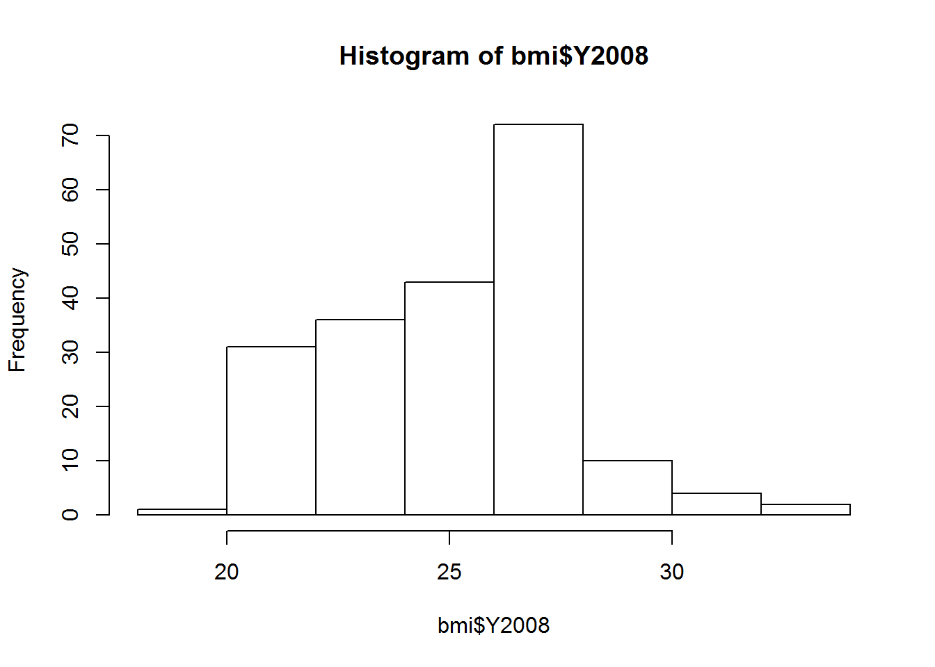
# Scatter plot comparing BMIs from 1980 to those from 2008
plot(bmi$Y1980,bmi$Y2008)
因此有 time-dependency.
3 拆分和合并列
参考 Carchedi (2016a)
suppressMessages(library(tidyverse))
mtcars %>%
    head %>%
    unite(total,mpg,cyl,sep='-')
mtcars %>%
head %>%
unite(total,mpg,cyl,sep='-') %>%
separate(total, into = c('mpg','cyl'),sep = '-')4 R 数据类型
参考 Carchedi (2016a)
4.1 五大数据类型
# Make this evaluate to "character"
class("TRUE")
## [1] "character"# Make this evaluate to "numeric"
class(8484.00);class(as.numeric(TRUE))## [1] "numeric"## [1] "numeric"# Make this evaluate to "integer"
class(99L)## [1] "integer"# Make this evaluate to "factor"
class(factor("factor"))## [1] "factor"# Make this evaluate to "logical"
class(as.logical(0))## [1] "logical"integer 需要加上L
4.2 缺失值和特殊值定义
缺失值,可随机,但是完全这样假设也是不妥的,需要看实际情况。
NA## [1] NA无限大值,一般认为是异常值,需要剔除。
Inf## [1] Inf1/0## [1] Inf33333^33333## [1] InfNaN 一般考虑做成一个变量,比如分类变量。
NaN## [1] NaN0/0## [1] NaN1/0 - 1/0## [1] NaNa <- c(NA,Inf,NaN)
a## [1] NA Inf NaNany(is.na(a))## [1] TRUEany(is.infinite(a))## [1] TRUEany(is.nan(a))## [1] TRUEsum(is.na(a)) # NaN \in NA## [1] 2sum(is.infinite(a))## [1] 1sum(is.nan(a))## [1] 14.3 detect NA
complete.cases是 rowwise的。
suppressMessages(library(tidyverse))
complete.cases(mtcars) %>% length
## [1] 32mtcars %>% dim## [1] 32 114.3.1 detect outlier
suppressMessages(library(tidyverse))
students3 <- read_csv("datasets/students_with_dates.csv")
hist(students3$absences)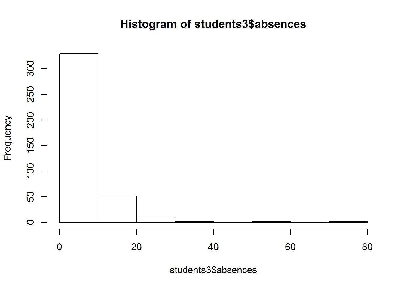
hist(students3$absences,right = F)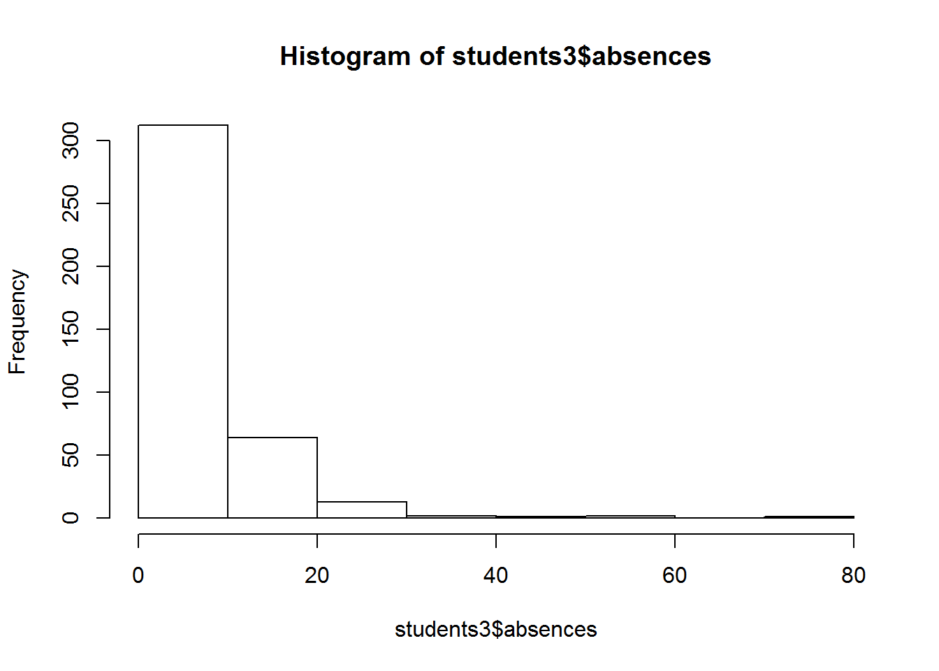
boxplot(students3$absences)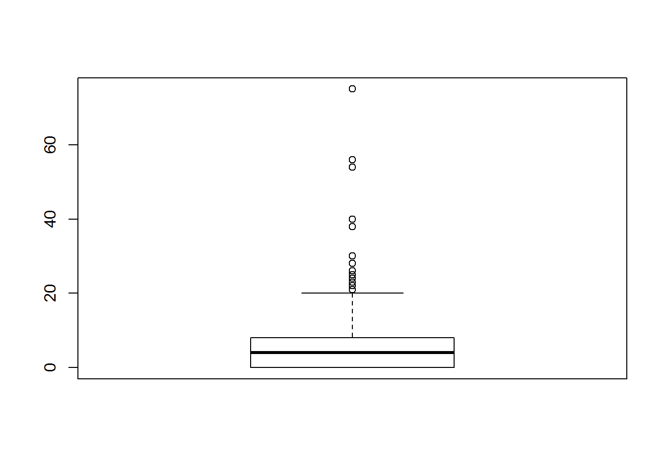
right
logical; if TRUE, the histogram cells are right-closed (left open) intervals.
这里的图,主要是展示 idea。
5 异常值检查
参考 Carchedi (2016a)
summary可以用于探查异常值。
max 和 min 是表现得地方。
library(magrittr)
c(-100,1:100) %>% summary()
## Min. 1st Qu. Median Mean 3rd Qu. Max.
## -100.00 25.00 50.00 49.01 75.00 100.00可以发现 1st Qu. 都有 25 但是 Min. 有 -100,应该就是极值。
6 缺失值检查
6.1 一般情况
参考 Carchedi (2016a)
参考DataCamp
as.numeric("chr")## [1] NANAs introduced by coercion报错的意思理解了。
当把一个 chr 变成 numeric,只会反馈 NA 了。
6.2 在df的情况
参考 Carchedi (2016a)
library(readr)
weather <- read_rds("datasets/weather.rds")
这是最快探查 NA 的方式,函数也非常的 base,易于调动。
library(magrittr)
sum(is.na(weather))
## [1] 820summary(weather)## X year month measure
## Min. : 1.00 Min. :2014 Min. : 1.000 Length:286
## 1st Qu.: 72.25 1st Qu.:2015 1st Qu.: 4.000 Class :character
## Median :143.50 Median :2015 Median : 7.000 Mode :character
## Mean :143.50 Mean :2015 Mean : 6.923
## 3rd Qu.:214.75 3rd Qu.:2015 3rd Qu.:10.000
## Max. :286.00 Max. :2015 Max. :12.000
## X1 X2 X3
## Length:286 Length:286 Length:286
## Class :character Class :character Class :character
## Mode :character Mode :character Mode :character
##
##
##
## X4 X5 X6
## Length:286 Length:286 Length:286
## Class :character Class :character Class :character
## Mode :character Mode :character Mode :character
##
##
##
## X7 X8 X9
## Length:286 Length:286 Length:286
## Class :character Class :character Class :character
## Mode :character Mode :character Mode :character
##
##
##
## X10 X11 X12
## Length:286 Length:286 Length:286
## Class :character Class :character Class :character
## Mode :character Mode :character Mode :character
##
##
##
## X13 X14 X15
## Length:286 Length:286 Length:286
## Class :character Class :character Class :character
## Mode :character Mode :character Mode :character
##
##
##
## X16 X17 X18
## Length:286 Length:286 Length:286
## Class :character Class :character Class :character
## Mode :character Mode :character Mode :character
##
##
##
## X19 X20 X21
## Length:286 Length:286 Length:286
## Class :character Class :character Class :character
## Mode :character Mode :character Mode :character
##
##
##
## X22 X23 X24
## Length:286 Length:286 Length:286
## Class :character Class :character Class :character
## Mode :character Mode :character Mode :character
##
##
##
## X25 X26 X27
## Length:286 Length:286 Length:286
## Class :character Class :character Class :character
## Mode :character Mode :character Mode :character
##
##
##
## X28 X29 X30
## Length:286 Length:286 Length:286
## Class :character Class :character Class :character
## Mode :character Mode :character Mode :character
##
##
##
## X31
## Length:286
## Class :character
## Mode :character
##
##
## weather[!complete.cases(weather), ] %>% head7 变量和值的命名
参考 Carchedi (2016a)
Because the period (
.) has special meaning in certain situations, we generally recommend using underscores (·) to separate words in variable names. We also prefer all lowercase letters so that no one has to remember which letters are uppercase or lowercase. DataCamp
命名避免使用.,而使用_,统一小写。
Finally, the events column (renamed to be all lowercase in the first instruction) contains an empty string (
"") for any day on which there was no significant weather event such as rain, fog, a thunderstorm, etc. However, if it’s the first time you’re seeing these data, it may not be obvious that this is the case, so it’s best for us to be explicit and replace the empty strings with something more meaningful. DataCamp
文本值不要写"",以清晰表示,如无。
8 which函数的使用
参考 Carchedi (2016a)
反馈一个 TRUE or FALSE vector 中,TRUE 的 index。
library(magrittr)
c(TRUE,FALSE,TRUE)
## [1] TRUE FALSE TRUEc(TRUE,FALSE,TRUE) %>% which## [1] 1 3(!c(TRUE,FALSE,TRUE)) %>% which(.)## [1] 2which.max(1:10)## [1] 10which.min(1:10)## [1] 19 案例
9.1 Online Ticket Sales Data
参考 Carchedi (2016b)
An easy way to get rid of unnecessary columns is to create a vector containing the column indices you want to keep, then subset the data based on that vector using single bracket subsetting. DataCamp
suppressMessages(library(tidyverse))
sales <- read_csv("datasets/sales.csv")[,-1]
R 中保留字段,偏工程的方式,和 Python 类似。
keep <- 5:(ncol(sales) - 15)
sales3 <- sales[,keep]
# Load tidyr
library(tidyr)
# Split event_date_time: sales4
sales4 <- separate(sales3, event_date_time,
into = c('event_dt','event_time'), sep = ' ')
# Split sales_ord_create_dttm: sales5
sales5 <- separate(sales4, sales_ord_create_dttm,
into = c('ord_create_dt','ord_create_time'), sep = ' ')在 Import 数据时的报错
Missing column names filled in: 'X1' [1]Parsed with column specification:
cols(
  .default = col_character(),
  X1 = col_double(),
  tickets_purchased_qty = col_double(),
  trans_face_val_amt = col_double(),
  event_date_time = col_datetime(format = ""),
  event_dt = col_date(format = ""),
  sales_ord_create_dttm = col_datetime(format = ""),
  sales_ord_tran_dt = col_date(format = ""),
  print_flg = col_logical(),
  dist_to_ven = col_double()
)
See spec(...) for full column specifications.
4 parsing failures.
 row                   col   expected actual                 file
2516 sales_ord_create_dttm date like    NULL 'datasets/sales.csv'
3863 sales_ord_create_dttm date like    NULL 'datasets/sales.csv'
4082 sales_ord_create_dttm date like    NULL 'datasets/sales.csv'
4183 sales_ord_create_dttm date like    NULL 'datasets/sales.csv'
这里进行查看。
# Define an issues vector
issues <- c(2516,3863,4082,4183)

# Print values of sales_ord_create_dttm at these indices
sales3$sales_ord_create_dttm[issues]
## [1] NA NA NA NA# Print a well-behaved value of sales_ord_create_dttm
sales3$sales_ord_create_dttm[2517]## [1] "2013-08-04 23:07:19 UTC"原来是空值,该数据类型应该为时间。
# Load stringr
library(stringr)

# Find columns of sales5 containing "dt": date_cols
date_cols <- str_detect(names(sales5),"dt")

# Load lubridate
library(lubridate)

# Coerce date columns into Date objects
sales5[, date_cols] <- lapply(sales5[,date_cols], ymd)
产生报警
2892 failed to parse. 101 failed to parse. 424 failed to parse.# Find date columns (don't change)
date_cols <- str_detect(names(sales5), "dt")
# Create logical vectors indicating missing values (don't change)
missing <- lapply(sales5[, date_cols], is.na)
# Create a numerical vector that counts missing values: num_missing
num_missing <- sapply(missing,sum)
# Print num_missing
num_missing## event_dt presale_dt onsale_dt ord_create_dt
## 0 2892 101 4
## sales_ord_tran_dt print_dt
## 0 424这里解释了产生 failed to parse 报错的原因。
这里每段任务都模块化,而非 pipeline 随意的合并。
9.2 Boston’s public transit system
参考 Carchedi (2016b)
library(readxl)
mbta <- read_excel("datasets/mbta.xlsx",skip = 1)
第一行是表格标题。
mbta[,1:10]All Modes by Qtrit is a quarterly average of weekday MBTA ridership. Since this dataset tracks monthly average ridership, you’ll remove that row.- the 7th row (
Pct Chg / Yr) and the 11th row (TOTAL) are not really observations as much as they are analysis.
# Remove rows 1, 7, and 11 of mbta: mbta2
mbta2 <- mbta[-c(1,7,11),]

# Remove the first column of mbta2: mbta3
mbta3 <- mbta2[,-1]
# Load tidyr
library(tidyr)
# Gather columns of mbta3: mbta4
mbta4 <- gather(mbta3, month, thou_riders, -mode)
# View the head of mbta4
head(mbta4)9.3 World Food Data
参考 Carchedi (2016b)
# Load data.table
library(data.table)

# Import food.csv as a data frame: food
food <- fread("datasets/food.csv",data.table = F)select参数看似和 dplyr 包类似,实际上是为了读取大数据集设计的,可以单独看若干变量,减少 import 数据量。
因为 R 在输入和输出时,耗费资源很大。
参考
github
class(food)## [1] "data.frame"因为加了参数data.table = F
参考文献
Carchedi, Nick. 2016a. “Cleaning Data in R.” 2016. https://www.datacamp.com/courses/cleaning-data-in-r.
———. 2016b. “Importing & Cleaning Data in R: Case Studies.” 2016. https://www.datacamp.com/courses/importing-cleaning-data-in-r-case-studies.