R 数据导入学习笔记
2020-05-29
- 使用 RMarkdown 的
child参数,进行文档拼接。 - 这样拼接以后的笔记方便复习。
- 相关问题提交到 GitHub
1 安装 R 和 RStudio
R是底层软件,RStudio是使用它比较方便的软件,界面友好。
1.0.0.1 安装R
- 打开网址The Comprehensive R Archive Network
- 选择Download R for Windows
- 选择install R for the first time
- 选择Download R 3.x.x for Windows。
- 然后点开对应的
.exe文件,安装好。
1.0.0.2 RStudio
- 打开网址RStudio – Open source and enterprise-ready professional software for R
- 下载RStudio,Shiny和R Packages两个暂时不用管。
- 选择Free的第一个Download RStudio – RStudio。
- 然后点开对应的
.exe文件,安装好。 - 安装好了,就可以开始最简单的录入,EDA等等简单,后面再搞回归那些R弄起来都很简单,有现成的包。
1.0.0.3 安装重要的包
打开 RStudio
右上角,点击新建项目,选路径,选新项目。 给名字(不要中文),点击 Create Proj \(\to\) Tools \(\to\) Global Options \(\to\) Packages \(\to\) Mirror \(\to\) 选一个中国的镜像,选清华
安装包 点
- Tools \(\to\) Install Packages \(\to\) ‘tidyverse’ \(\to\) Install
- Tools \(\to\) Install Packages \(\to\) ‘rebus’ \(\to\) Install
- Tools \(\to\) Install Packages \(\to\) ‘rmarkdown’ \(\to\) Install
左上角
R Notebook \(\to\) 新建一个Rmd \(\to\) Ctrl + S Save
快捷键 Ctrl + Alt + I 新建 chunk
快捷键 Shift + Ctrl + Enter run
再新建一个 Chunk Ctrl + Alt + I
2 导入数据 1
参考 Schouwenaars (2016a)
2.1 stringsAsFactors = FALSE
Import strings as categorical variables?
2.2 txt 文件读取
# Import hotdogs.txt: hotdogs
hotdogs <- read.delim("datasets/hotdogs.txt",sep = '\t',header = F)

# Summarize hotdogs
summary(hotdogs)
## V1 V2 V3
## Beef :20 Min. : 86.0 Min. :144.0
## Meat :17 1st Qu.:132.0 1st Qu.:362.5
## Poultry:17 Median :145.0 Median :405.0
## Mean :145.4 Mean :424.8
## 3rd Qu.:172.8 3rd Qu.:503.5
## Max. :195.0 Max. :645.0注意 sep = '\t'
## [1] "Beef\t186\t495" "Beef\t181\t477" "Beef\t176\t425" "Beef\t149\t322"
## [5] "Beef\t184\t482" "Beef\t190\t587"
\t 就是分割符号。
2.3 指定变量名称
可以指定对应的 column name
# Finish the read.delim() call
hotdogs <- read.delim("datasets/hotdogs.txt", header = F, col.names = c("type", "calories", 'sodium'))

# Select the hot dog with the least calories: lily
lily <- hotdogs[which.min(hotdogs$calories), ]

# Select the observation with the most sodium: tom
tom <- hotdogs[which.max(hotdogs$sodium), ]

# Print lily and tom
lilywhich.max和which.min,反馈 index,类似于
\(\arg\max_{\text{index}}\text{variable}\)。
参考 Schouwenaars (2016a)
2.4 skip and n_max
## [1] "hotdogs.txt"               "mtcars-with-comments.xlsx"
## [3] "potatoes.csv"              "potatoes.txt"
## [5] "swimming_pools.csv"        "urbanpop.xls"
## [7] "urbanpop.xlsx"
properties <- c("area", "temp", "size", "storage", "method",
"texture", "flavor", "moistness")
library(readr)
potatoes_fragment <- read_tsv("datasets/potatoes.txt",skip = 2, n_max = 3, col_names = properties)
potatoes_fragment其他的 read_* 也可以加上 n_max,触类旁通。
2.5 col_types
You can manually set the types with a string, where each character denotes the class of the column:
character,double,integer andlogical.
这是 R 的四种数据。
# readr is already loaded

# Column names
properties <- c("area", "temp", "size", "storage", "method",
                "texture", "flavor", "moistness")

# Import all data, but force all columns to be character: potatoes_char
potatoes_char <- read_tsv("datasets/potatoes.txt", col_types = "cccccccc", col_names = properties,
                          n_max = 3
                          )

# Print out structure of potatoes_char
str(potatoes_char)
## Classes 'spec_tbl_df', 'tbl_df', 'tbl' and 'data.frame': 3 obs. of 8 variables:
## $ area : chr "1" "1" "1"
## $ temp : chr "1" "1" "1"
## $ size : chr "1" "1" "1"
## $ storage : chr "1" "1" "1"
## $ method : chr "1" "2" "3"
## $ texture : chr "2.9" "2.3" "2.5"
## $ flavor : chr "3.2" "2.5" "2.8"
## $ moistness: chr "3.0" "2.6" "2.8"
## - attr(*, "spec")=
## .. cols(
## .. area = col_character(),
## .. temp = col_character(),
## .. size = col_character(),
## .. storage = col_character(),
## .. method = col_character(),
## .. texture = col_character(),
## .. flavor = col_character(),
## .. moistness = col_character()
## .. )参考 Schouwenaars (2016a)
- readxl by Hadley Wickham
- gdata by Gregory Warnes
2.6 批量读取 excel
library(readxl)
pop_list <- lapply(excel_sheets("datasets/urbanpop.xlsx"),
                   read_excel,path = "datasets/urbanpop.xlsx"
                   )
str(pop_list)
## List of 3
## $ :Classes 'tbl_df', 'tbl' and 'data.frame': 209 obs. of 8 variables:
## ..$ country: chr [1:209] "Afghanistan" "Albania" "Algeria" "American Samoa" ...
## ..$ 1960 : num [1:209] 769308 494443 3293999 NA NA ...
## ..$ 1961 : num [1:209] 814923 511803 3515148 13660 8724 ...
## ..$ 1962 : num [1:209] 858522 529439 3739963 14166 9700 ...
## ..$ 1963 : num [1:209] 903914 547377 3973289 14759 10748 ...
## ..$ 1964 : num [1:209] 951226 565572 4220987 15396 11866 ...
## ..$ 1965 : num [1:209] 1000582 583983 4488176 16045 13053 ...
## ..$ 1966 : num [1:209] 1058743 602512 4649105 16693 14217 ...
## $ :Classes 'tbl_df', 'tbl' and 'data.frame': 209 obs. of 9 variables:
## ..$ country: chr [1:209] "Afghanistan" "Albania" "Algeria" "American Samoa" ...
## ..$ 1967 : num [1:209] 1119067 621180 4826104 17349 15440 ...
## ..$ 1968 : num [1:209] 1182159 639964 5017299 17996 16727 ...
## ..$ 1969 : num [1:209] 1248901 658853 5219332 18619 18088 ...
## ..$ 1970 : num [1:209] 1319849 677839 5429743 19206 19529 ...
## ..$ 1971 : num [1:209] 1409001 698932 5619042 19752 20929 ...
## ..$ 1972 : num [1:209] 1502402 720207 5815734 20263 22406 ...
## ..$ 1973 : num [1:209] 1598835 741681 6020647 20742 23937 ...
## ..$ 1974 : num [1:209] 1696445 763385 6235114 21194 25482 ...
## $ :Classes 'tbl_df', 'tbl' and 'data.frame': 209 obs. of 38 variables:
## ..$ country: chr [1:209] "Afghanistan" "Albania" "Algeria" "American Samoa" ...
## ..$ 1975 : num [1:209] 1793266 785350 6460138 21632 27019 ...
## ..$ 1976 : num [1:209] 1905033 807990 6774099 22047 28366 ...
## ..$ 1977 : num [1:209] 2021308 830959 7102902 22452 29677 ...
## ..$ 1978 : num [1:209] 2142248 854262 7447728 22899 31037 ...
## ..$ 1979 : num [1:209] 2268015 877898 7810073 23457 32572 ...
## ..$ 1980 : num [1:209] 2398775 901884 8190772 24177 34366 ...
## ..$ 1981 : num [1:209] 2493265 927224 8637724 25173 36356 ...
## ..$ 1982 : num [1:209] 2590846 952447 9105820 26342 38618 ...
## ..$ 1983 : num [1:209] 2691612 978476 9591900 27655 40983 ...
## ..$ 1984 : num [1:209] 2795656 1006613 10091289 29062 43207 ...
## ..$ 1985 : num [1:209] 2903078 1037541 10600112 30524 45119 ...
## ..$ 1986 : num [1:209] 3006983 1072365 11101757 32014 46254 ...
## ..$ 1987 : num [1:209] 3113957 1109954 11609104 33548 47019 ...
## ..$ 1988 : num [1:209] 3224082 1146633 12122941 35095 47669 ...
## ..$ 1989 : num [1:209] 3337444 1177286 12645263 36618 48577 ...
## ..$ 1990 : num [1:209] 3454129 1198293 13177079 38088 49982 ...
## ..$ 1991 : num [1:209] 3617842 1215445 13708813 39600 51972 ...
## ..$ 1992 : num [1:209] 3788685 1222544 14248297 41049 54469 ...
## ..$ 1993 : num [1:209] 3966956 1222812 14789176 42443 57079 ...
## ..$ 1994 : num [1:209] 4152960 1221364 15322651 43798 59243 ...
## ..$ 1995 : num [1:209] 4347018 1222234 15842442 45129 60598 ...
## ..$ 1996 : num [1:209] 4531285 1228760 16395553 46343 60927 ...
## ..$ 1997 : num [1:209] 4722603 1238090 16935451 47527 60462 ...
## ..$ 1998 : num [1:209] 4921227 1250366 17469200 48705 59685 ...
## ..$ 1999 : num [1:209] 5127421 1265195 18007937 49906 59281 ...
## ..$ 2000 : num [1:209] 5341456 1282223 18560597 51151 59719 ...
## ..$ 2001 : num [1:209] 5564492 1315690 19198872 52341 61062 ...
## ..$ 2002 : num [1:209] 5795940 1352278 19854835 53583 63212 ...
## ..$ 2003 : num [1:209] 6036100 1391143 20529356 54864 65802 ...
## ..$ 2004 : num [1:209] 6285281 1430918 21222198 56166 68301 ...
## ..$ 2005 : num [1:209] 6543804 1470488 21932978 57474 70329 ...
## ..$ 2006 : num [1:209] 6812538 1512255 22625052 58679 71726 ...
## ..$ 2007 : num [1:209] 7091245 1553491 23335543 59894 72684 ...
## ..$ 2008 : num [1:209] 7380272 1594351 24061749 61118 73335 ...
## ..$ 2009 : num [1:209] 7679982 1635262 24799591 62357 73897 ...
## ..$ 2010 : num [1:209] 7990746 1676545 25545622 63616 74525 ...
## ..$ 2011 : num [1:209] 8316976 1716842 26216968 64817 75207 ...2.7 gdata
# Load the gdata package
library(gdata)

# Import the second sheet of urbanpop.xls: urban_pop
urban_pop <- read.xls("urbanpop.xls", sheet = "1967-1974")

# Print the first 11 observations using head()
head(urban_pop, n = 11)
这里需要安装 perl,因此不推荐。
2.8 XLConnect
# urbanpop.xlsx is available in your working directory

# Load the XLConnect package
library(XLConnect)
library(XLConnectJars)

# Build connection to urbanpop.xlsx: my_book
my_book <- loadWorkbook("urbanpop.xlsx")

# Print out the class of my_book
class(my_book)
todo 需要安装 rJava。
可以增删 Excel,好;厉害。
# XLConnect is already available

# Build connection to urbanpop.xlsx
my_book <- loadWorkbook("urbanpop.xlsx")

# Add a worksheet to my_book, named "data_summary"
createSheet(my_book, "data_summary")

# Create data frame: summ
sheets <- getSheets(my_book)[1:3]
dims <- sapply(sheets, function(x) dim(readWorksheet(my_book, sheet = x)), USE.NAMES = FALSE)
summ <- data.frame(sheets = sheets,
                   nrows = dims[1, ],
                   ncols = dims[2, ])

# Add data in summ to "data_summary" sheet
writeWorksheet(my_book, summ, "data_summary")

# Save workbook as summary.xlsx
saveWorkbook(my_book, "summary.xlsx")
2.9 录入 excel
2.9.1 批量导入 excel
## List of 2
##  $ data_mtcars:'data.frame': 32 obs. of  11 variables:
##   ..$ mpg : num [1:32] 21 21 22.8 21.4 18.7 18.1 14.3 24.4 22.8 19.2 ...
##   ..$ cyl : num [1:32] 6 6 4 6 8 6 8 4 4 6 ...
##   ..$ disp: num [1:32] 160 160 108 258 360 ...
##   ..$ hp  : num [1:32] 110 110 93 110 175 105 245 62 95 123 ...
##   ..$ drat: num [1:32] 3.9 3.9 3.85 3.08 3.15 2.76 3.21 3.69 3.92 3.92 ...
##   ..$ wt  : num [1:32] 2.62 2.88 2.32 3.21 3.44 ...
##   ..$ qsec: num [1:32] 16.5 17 18.6 19.4 17 ...
##   ..$ vs  : num [1:32] 0 0 1 1 0 1 0 1 1 1 ...
##   ..$ am  : num [1:32] 1 1 1 0 0 0 0 0 0 0 ...
##   ..$ gear: num [1:32] 4 4 4 3 3 3 3 4 4 4 ...
##   ..$ carb: num [1:32] 4 4 1 1 2 1 4 2 2 4 ...
##  $ data_iris  :'data.frame': 150 obs. of  5 variables:
##   ..$ Sepal.Length: num [1:150] 5.1 4.9 4.7 4.6 5 5.4 4.6 5 4.4 4.9 ...
##   ..$ Sepal.Width : num [1:150] 3.5 3 3.2 3.1 3.6 3.9 3.4 3.4 2.9 3.1 ...
##   ..$ Petal.Length: num [1:150] 1.4 1.4 1.3 1.5 1.4 1.7 1.4 1.5 1.4 1.5 ...
##   ..$ Petal.Width : num [1:150] 0.2 0.2 0.2 0.2 0.2 0.4 0.3 0.2 0.2 0.1 ...
## ..$ Species : chr [1:150] "setosa" "setosa" "setosa" "setosa" ...## $result
## $result[[1]]
## NULL
##
##
## $error
## NULL但是导入出了问题。
2.10 导入 doc 表格
library(tidyverse)
library(tidycells)
fold <- system.file("extdata", "messy", package = "tidycells", mustWork = TRUE)
# this is because extension is intentionally given wrong
# while filename is actual identifier of the file type
fcsv <- list.files(fold, pattern = "^csv.", full.names = TRUE)[1]
basename(fcsv)
## [1] "csv.docx"表格存在 docx 文档中。
2.11 导出 excel
2.11.1 writexl 框架
参考 docs
Portable, light-weight data frame to xlsx exporter based on libxlsxwriter. No Java or Excel required.
这个包好在不需要调用 Java,比较轻量,点对点的解决导出 Excel 这一单一问题。
## [1] 84972.11.2 rio 框架
## [1] "data_mtcars" "data_iris"## $result
## [1] "mtcars.tsv.tar"
##
## $error
## NULL## $result
## [1] "mtcars.tsv.zip"
##
## $error
## NULLzip不支持在 Win 7 上,提交了问题 Github Issue 203。
压缩一组数据集
2.12 vroom 框架
rvoom 是 tidyverse 出品,因为维护有保证。
2.12.1 举例
library(vroom)
library(nycflights13)
source(here::here("R/load.R"))
flights_output_path <- here::here("output/flights.csv")## cols(
## year = col_double(),
## month = col_double(),
## day = col_double(),
## dep_time = col_double(),
## sched_dep_time = col_double(),
## dep_delay = col_double(),
## arr_time = col_double(),
## sched_arr_time = col_double(),
## arr_delay = col_double(),
## carrier = col_character(),
## flight = col_double(),
## tailnum = col_character(),
## origin = col_character(),
## dest = col_character(),
## air_time = col_double(),
## distance = col_double(),
## hour = col_double(),
## minute = col_double(),
## time_hour = col_datetime(format = "")
## )这里的思路很好,我一直觉得 read_* 这一步很好,因为很多时候 spec 的信息是不用展示的,因此用户不等不去除 msg 和 warning。
2.12.2 批量录入
2.12.3 导出压缩文件
## NA 7.87M第一个文件有21MB。 csv 文件诟病就是因为生成文件过大,压缩以后会小很多。
2.12.4 可读压缩文件
2.12.5 运行速度超过 data.table
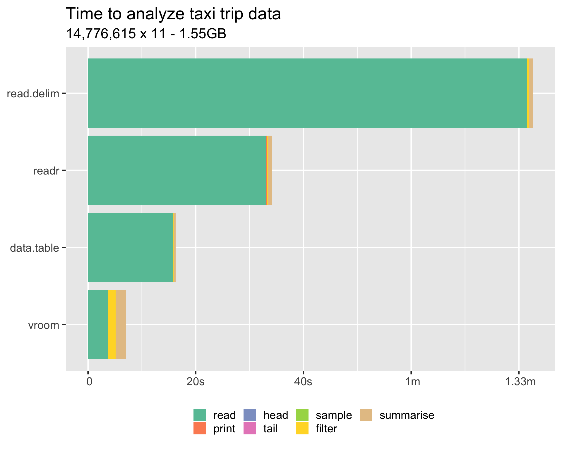
Figure 2.1: rvoom 速度超过 data.table
而且我们已知 data.table 的速度是超过 pandas 的。
2.13 其他
2.13.1 excel 读取特定行的思路
一般可以借助 read_excel 的两个参数
skip,但是如果需要提出的是第二行之后的某一行,这个参数失效range,这个太过于定制化,限定了第几行和第几列,不利于批量导入。
如表格,数据的问题是第一行是解释,需要删除,只需要选择第二行开始的数据,可以做如下处理。
2.13.2 read_table直接复制粘贴读取表格
library(readr)
read_table(
"name age      start  week1  week2  week3
Anne   35 2014-03-27 100/80 100/75 120/90
Ben    41 2014-03-09 110/65 100/65 135/70
Carl   33 2014-04-02 125/80   <NA>   <NA>
",na = "<NA>"
)
注意粘贴表格的缩进。 比如 有时候RStudio Community 和 Stack Overflow 上的例子数据是直接复制粘贴的,就可以这么操作。
3 导入数据 2
3.1 连接数据库
参考 Schouwenaars (2016b)
todo 如何设置 Impala 的
… you need different packages depending on the database you want to connect to. All of these packages do this in a uniform way, as specified in the
DBIpackage.
# Load the DBI package
library(DBI)

# Edit dbConnect() call
con <- dbConnect(RMySQL::MySQL(),
                 dbname = "tweater",
                 host = "courses.csrrinzqubik.us-east-1.rds.amazonaws.com",
                 port = 3306,
                 user = "student",
password = "datacamp")## [1] "MySQLConnection"
## attr(,"package")
## [1] "RMySQL"## chr [1:3] "comments" "tweats" "users"Good!
dbListTables()can be very useful to get a first idea about the contents of your database.
类似于 str 看下数据表的 column
目前三张表,进行一起阅读。
## [[1]]
##      id tweat_id user_id            message
## 1  1022       87       7              nice!
## 2  1000       77       7             great!
## 3  1011       49       5            love it
## 4  1012       87       1   awesome! thanks!
## 5  1010       88       6              yuck!
## 6  1026       77       4      not my thing!
## 7  1004       49       1  this is fabulous!
## 8  1030       75       6           so easy!
## 9  1025       88       2             oh yes
## 10 1007       49       3           serious?
## 11 1020       77       1 couldn't be better
## 12 1014       77       1       saved my day
##
## [[2]]
##   id user_id
## 1 75       3
## 2 88       4
## 3 77       6
## 4 87       5
## 5 49       1
## 6 24       7
##                                                                  post
## 1                                       break egg. bake egg. eat egg.
## 2                           wash strawberries. add ice. blend. enjoy.
## 3                       2 slices of bread. add cheese. grill. heaven.
## 4               open and crush avocado. add shrimps. perfect starter.
## 5 nachos. add tomato sauce, minced meat and cheese. oven for 10 mins.
## 6                              just eat an apple. simply and healthy.
##         date
## 1 2015-09-05
## 2 2015-09-14
## 3 2015-09-21
## 4 2015-09-22
## 5 2015-09-22
## 6 2015-09-24
##
## [[3]]
##   id      name     login
## 1  1 elisabeth  elismith
## 2  2      mike     mikey
## 3  3      thea   teatime
## 4  4    thomas tomatotom
## 5  5    oliver olivander
## 6  6      kate  katebenn
## 7  7    anjali    lianja
这三张表的逻辑是
tweat表示 tweeter 的一个帖子tweat_id是一个帖子的id- 回复
awesome! thanks!的帖子是tweat_id = 87
- 查看第二张表,是
user_id = 5发的 - 查看第三张表,是
name = oliver发的
todo RMarkdown SQL chunk 如何操作。
参考 Schouwenaars (2016b)
3.2 query
# Connect to the database
library(DBI)
con <- dbConnect(RMySQL::MySQL(),
                 dbname = "tweater",
                 host = "courses.csrrinzqubik.us-east-1.rds.amazonaws.com",
                 port = 3306,
                 user = "student",
                 password = "datacamp")

# Import tweat_id column of comments where user_id is 1: elisabeth
elisabeth <- dbGetQuery(con, "select tweat_id from comments where user_id = 1")

# Print elisabeth
elisabeth
参考 rmarkdown
| tweat_id |
|---|
| 87 |
| 49 |
| 77 |
| 77 |
3.3 fetch
… but make sure to remember this technique when you’re struggling with huge databases! DataCamp
## $statement
## [1] "SELECT * FROM comments WHERE user_id > 4"
##
## $isSelect
## [1] 1
##
## $rowsAffected
## [1] -1
##
## $rowCount
## [1] 0
##
## $completed
## [1] 0
##
## $fieldDescription
## $fieldDescription[[1]]
## NULL## [1] TRUEres只是一个命令,反馈的和 dbGetQuery 不同。
todo 查看 RODBC 有没有类似的函数。 https://cran.r-project.org/web/packages/RODBC/RODBC.pdf 需要自己看。
参考 Schouwenaars (2016b)
3.4 web excel
对于在 Web 上的 Excel
- gdata 可以直接连接
- readxl 必须先下载后才能连接,使用
download.file函数,必须指定dest.file参数
具体参考 Reference。
3.5 web RData
You can load data from an RData file using the load() function, but this function does not accept a URL string as an argument. In this exercise, you’ll first download the RData file securely, and then import the local data file. DataCamp
也需要下载。
# https URL to the wine RData file.
url_rdata <- "https://s3.amazonaws.com/assets.datacamp.com/production/course_1478/datasets/wine.RData"

# Download the wine file to your working directory
download.file(url_rdata,"wine_local.RData")

# Load the wine data into your workspace using load()
load("wine_local.RData")

# Print out the summary of the wine data
wine
trying URL 'https://s3.amazonaws.com/assets.datacamp.com/production/course_1478/datasets/wine.RData'
InternetOpenUrl failed: '�����������������'Error in download.file(url_rdata, "wine_local.RData") :
cannot open URL 'https://s3.amazonaws.com/assets.datacamp.com/production/course_1478/datasets/wine.RData'报错。
3.6 Get 请求
参考 Schouwenaars (2016b)
Downloading a file from the Internet means sending a GET request and receiving the file you asked for. Internally, all the previously discussed functions use a GET request to download files.
这是 GET 请求最直观的定义。 通过网页链接下载文件,这都算是 GET 请求。
# Load the httr package
library(httr)

# Get the url, save response to resp
url <- "http://www.example.com/"
resp <- GET(url)


# Print resp
resp
## Response [http://www.example.com/]
## Date: 2020-05-29 03:04
## Status: 200
## Content-Type: text/html; charset=UTF-8
## Size: 1.26 kB
## <!doctype html>
## <html>
## <head>
## <title>Example Domain</title>
##
## <meta charset="utf-8" />
## <meta http-equiv="Content-type" content="text/html; charset=utf-8" />
## <meta name="viewport" content="width=device-width, initial-scale=1" />
## <style type="text/css">
## body {
## ...resp 的内容,类似于 view source 出来的网页源代码。
library(httr)

# Get the url
url <- "http://www.omdbapi.com/?apikey=72bc447a&t=Annie+Hall&y=&plot=short&r=json"


# Print resp
resp <- GET(url)
resp
## Response [http://www.omdbapi.com/?apikey=72bc447a&t=Annie+Hall&y=&plot=short&r=json]
## Date: 2020-05-29 03:04
## Status: 200
## Content-Type: application/json; charset=utf-8
## Size: 910 B## [1] "{\"Title\":\"Annie Hall\",\"Year\":\"1977\",\"Rated\":\"PG\",\"Released\":\"20 Apr 1977\",\"Runtime\":\"93 min\",\"Genre\":\"Comedy, Romance\",\"Director\":\"Woody Allen\",\"Writer\":\"Woody Allen, Marshall Brickman\",\"Actors\":\"Woody Allen, Diane Keaton, Tony Roberts, Carol Kane\",\"Plot\":\"Neurotic New York comedian Alvy Singer falls in love with the ditzy Annie Hall.\",\"Language\":\"English, German\",\"Country\":\"USA\",\"Awards\":\"Won 4 Oscars. Another 26 wins & 8 nominations.\",\"Poster\":\"https://m.media-amazon.com/images/M/MV5BZDg1OGQ4YzgtM2Y2NS00NjA3LWFjYTctMDRlMDI3NWE1OTUyXkEyXkFqcGdeQXVyMjUzOTY1NTc@._V1_SX300.jpg\",\"Ratings\":[{\"Source\":\"Internet Movie Database\",\"Value\":\"8.0/10\"},{\"Source\":\"Rotten Tomatoes\",\"Value\":\"98%\"},{\"Source\":\"Metacritic\",\"Value\":\"92/100\"}],\"Metascore\":\"92\",\"imdbRating\":\"8.0\",\"imdbVotes\":\"245,897\",\"imdbID\":\"tt0075686\",\"Type\":\"movie\",\"DVD\":\"N/A\",\"BoxOffice\":\"N/A\",\"Production\":\"N/A\",\"Website\":\"N/A\",\"Response\":\"True\"}"## $Title
## [1] "Annie Hall"
##
## $Year
## [1] "1977"
##
## $Rated
## [1] "PG"
##
## $Released
## [1] "20 Apr 1977"
##
## $Runtime
## [1] "93 min"
##
## $Genre
## [1] "Comedy, Romance"
##
## $Director
## [1] "Woody Allen"
##
## $Writer
## [1] "Woody Allen, Marshall Brickman"
##
## $Actors
## [1] "Woody Allen, Diane Keaton, Tony Roberts, Carol Kane"
##
## $Plot
## [1] "Neurotic New York comedian Alvy Singer falls in love with the ditzy Annie Hall."
##
## $Language
## [1] "English, German"
##
## $Country
## [1] "USA"
##
## $Awards
## [1] "Won 4 Oscars. Another 26 wins & 8 nominations."
##
## $Poster
## [1] "https://m.media-amazon.com/images/M/MV5BZDg1OGQ4YzgtM2Y2NS00NjA3LWFjYTctMDRlMDI3NWE1OTUyXkEyXkFqcGdeQXVyMjUzOTY1NTc@._V1_SX300.jpg"
##
## $Ratings
## $Ratings[[1]]
## $Ratings[[1]]$Source
## [1] "Internet Movie Database"
##
## $Ratings[[1]]$Value
## [1] "8.0/10"
##
##
## $Ratings[[2]]
## $Ratings[[2]]$Source
## [1] "Rotten Tomatoes"
##
## $Ratings[[2]]$Value
## [1] "98%"
##
##
## $Ratings[[3]]
## $Ratings[[3]]$Source
## [1] "Metacritic"
##
## $Ratings[[3]]$Value
## [1] "92/100"
##
##
##
## $Metascore
## [1] "92"
##
## $imdbRating
## [1] "8.0"
##
## $imdbVotes
## [1] "245,897"
##
## $imdbID
## [1] "tt0075686"
##
## $Type
## [1] "movie"
##
## $DVD
## [1] "N/A"
##
## $BoxOffice
## [1] "N/A"
##
## $Production
## [1] "N/A"
##
## $Website
## [1] "N/A"
##
## $Response
## [1] "True"… the
content()function by default, if you don’t specify theasargument, figures out what type of data you’re dealing with and parses it for you.
as 一般不用设置,httr 的函数会自动判断。
httrconverts the JSON response body automatically to an R list
根据 Reference 的介绍, JSON 格式主要是两种组成方式,数列和对象。
两个输入数据如下,
{"info_age": 28, "name": "张三"}
{"info_age": 28, "name": "张三", "sex": "f"}
因此,可以判断,
- 数据应该以数列方式连接,因为数据类型一致,约等于
[{"info_age": 28, "name": "张三"}, {"info_age": 28, "name": "张三", "sex": "f"}]- 每个输入的元素内部变量数据类型不一致,但是不存在嵌套,可以转换成一个表格(矩阵不行),如下。
## {
##     "info_age": 28,
##     "name": "张三",
##     "sex": "f"
## }
##
因此,对于每个输入可以用同一函数处理,每个输入内部转换成一个 data.frame。 可以参考github。
本文在
[{"info_age": 28, "name": "张三"}, {"info_age": 28, "name": "张三", "sex": "f"]基础上,进行第二种方式处理。
这是更加简易的方式。
3.7 JSON
3.7.1 Defination
JSON — short for JavaScript Object Notation — is a format for sharing data. As its name suggests, JSON is derived from the JavaScript programming language, but it’s available for use by many other languages.
JSON is a lightweight text-based open standard data-interchange format. It is human readable. A lot of data on the web are not available in tabular format. And sometimes you don’t want to go to the website such as https://ihis.ipums.org/ihis/ and select the data you need. Instead data are dynamically provided by a web server to a web browser based on queries or requests and you can write a program to select and download the data.
Example: https://www.bloomberg.com/markets/api/bulk-time-series/price/GOOGL%3AUS?timeFrame=1_MONTH
- This is a smart code, I will use it. Because I avoid repeating installation.
Let’s break that down a bit:
Each object is surrounded by curly braces. The entire JSON response is itself an object so it is surrounded by braces. It contains objects: id, dateTimeRanges, price, timeZoneObject and so on.
price is a JSON inside a JSON. Data can be nested within the JSON format by using square brackets
[ ].Each object may have multiple name/value pairs separated by a comma. Name/value pairs may represent a single value (as with “id”) or multiple values in an array (as with “price”). Note the use of the colon separating the name from the associated value(s).
As you can see, JSON has a very simple structure and format, once you’re able to break it down.
3.7.2 Application
Create a dataframe stations using citibike to produce a map of stations.
You will then use stations here:
map <- leaflet(stations)
map <- addTiles(map)
map <-
  addMarkers(
    map,
    stations$stationBeanList.longitude,
    stations$stationBeanList.latitude,
    popup = stations$stationBeanList.stationName
  )
map
Error in stations$longitude : $ operator is invalid for atomic vectorsmay happen.
## [1] TRUE参考 Schouwenaars (2016b)
jsonlite 取名取自 SQLite。
# Load the jsonlite package
library(jsonlite)
library(glue)

# wine_json is a JSON
wine_json <- '{"name":"Chateau Migraine", "year":1997, "alcohol_pct":12.4, "color":"red", "awarded":false}'
wine_json_bracket <- glue('[{wine_json}]')

# Convert wine_json into a list: wine
wine <- fromJSON(wine_json)
wine_bracket <- fromJSON(wine_json_bracket)

# Print structure of wine
str(wine)
## List of 5
## $ name : chr "Chateau Migraine"
## $ year : int 1997
## $ alcohol_pct: num 12.4
## $ color : chr "red"
## $ awarded : logi FALSE## 'data.frame': 1 obs. of 5 variables:
## $ name : chr "Chateau Migraine"
## $ year : int 1997
## $ alcohol_pct: num 12.4
## $ color : chr "red"
## $ awarded : logi FALSEJSON is built on two structures: objects and arrays. DataCamp
如上的举例,我们发现,
- 以
{}为总结构,因此反馈是一个list。 []帮助识别成表格。
以下进行系统的解释。
3.7.3 JSON Structure
## [1] "integer"## [1] "list"## [1] "matrix"## [1] "data.frame"如果元素在一个 array 中,例如,[1, 2, 3, 4, 5, 6],那么数据类型一致,可以放入一个 vector 或者 matrix 中,以区别于 data.frame 和 list。
这点可以参考 Reference
如果元素在一个 {} 中,系统默认为可以是不同的数据类型,因此处理成 data.frame 中的两列,或者 list。
通过以上的解释,当 toJSON 把 R 中的四大格式
- vectors
- matrix
- data.frame
- list
转换成 json 时,也有理可据。
3.7.4 prettify or minify JSON
JSONs can come in different formats. Take these two JSONs, that are in fact exactly the same: the first one is in a minified format, the second one is in a pretty format with indentation, whitespace and new lines: DataCamp
JSON 一般由两种格式
- 一种是 minified 格式,非常紧凑,少空格、缩进,利于读取
- 一种是 prettied 格式,有空格、缩进,利于读取
# pretty_json <- prettify(toJSON(mtcars[1:5,1:2]))
pretty_json <- toJSON(mtcars[1:5,1:2], pretty = TRUE)

# Print pretty_json
pretty_json
## [
## {
## "mpg": 21,
## "cyl": 6,
## "_row": "Mazda RX4"
## },
## {
## "mpg": 21,
## "cyl": 6,
## "_row": "Mazda RX4 Wag"
## },
## {
## "mpg": 22.8,
## "cyl": 4,
## "_row": "Datsun 710"
## },
## {
## "mpg": 21.4,
## "cyl": 6,
## "_row": "Hornet 4 Drive"
## },
## {
## "mpg": 18.7,
## "cyl": 8,
## "_row": "Hornet Sportabout"
## }
## ]## [{"mpg":21,"cyl":6,"_row":"Mazda RX4"},{"mpg":21,"cyl":6,"_row":"Mazda RX4 Wag"},{"mpg":22.8,"cyl":4,"_row":"Datsun 710"},{"mpg":21.4,"cyl":6,"_row":"Hornet 4 Drive"},{"mpg":18.7,"cyl":8,"_row":"Hornet Sportabout"}]3.7.5 fromJSON`可以识别链接
# Definition of quandl_url
quandl_url <- "https://www.quandl.com/api/v3/datasets/WIKI/FB/data.json?auth_token=i83asDsiWUUyfoypkgMz"

# Import Quandl data: quandl_data
quandl_data <- fromJSON(quandl_url)

# Print structure of quandl_data
str(quandl_data)
## List of 1
## $ dataset_data:List of 10
## ..$ limit : NULL
## ..$ transform : NULL
## ..$ column_index: NULL
## ..$ column_names: chr [1:13] "Date" "Open" "High" "Low" ...
## ..$ start_date : chr "2012-05-18"
## ..$ end_date : chr "2018-03-27"
## ..$ frequency : chr "daily"
## ..$ data : chr [1:1472, 1:13] "2018-03-27" "2018-03-26" "2018-03-23" "2018-03-22" ...
## ..$ collapse : NULL
## ..$ order : NULL## $name
## [1] "Chateau Migraine"
##
## $year
## [1] 1997
##
## $alcohol_pct
## [1] 12.4
##
## $color
## [1] "red"
##
## $awarded
## [1] FALSE参考 Schouwenaars (2016b)
3.8 stata
研究下部分参数
# foreign is already loaded

# Specify the file path using file.path(): path
path <- file.path("datasets","edequality.dta")

# Create and print structure of edu_equal_1
edu_equal_1 <- read.dta(path)
str(edu_equal_1)
## 'data.frame': 12214 obs. of 27 variables:
## $ hhid : num 1 1 1 2 2 3 4 4 5 6 ...
## $ hhweight : num 627 627 627 627 627 ...
## $ location : Factor w/ 2 levels "urban location",..: 1 1 1 1 1 2 2 2 1 1 ...
## $ region : Factor w/ 9 levels "Sofia city","Bourgass",..: 8 8 8 9 9 4 4 4 8 8 ...
## $ ethnicity_head : Factor w/ 4 levels "Bulgaria","Turks",..: 2 2 2 1 1 1 1 1 1 1 ...
## $ age : num 37 11 8 73 70 75 79 80 82 83 ...
## $ gender : Factor w/ 2 levels "male","female": 2 2 1 1 2 1 1 2 2 2 ...
## $ relation : Factor w/ 9 levels "head ",..: 1 3 3 1 2 1 1 2 1 1 ...
## $ literate : Factor w/ 2 levels "no","yes": 1 2 2 2 2 2 2 2 2 2 ...
## $ income_mnt : num 13.3 13.3 13.3 142.5 142.5 ...
## $ income : num 160 160 160 1710 1710 ...
## $ aggregate : num 1042 1042 1042 3271 3271 ...
## $ aggr_ind_annual : num 347 347 347 1635 1635 ...
## $ educ_completed : int 2 4 4 4 3 3 3 3 4 4 ...
## $ grade_complete : num 4 3 0 3 4 4 4 4 5 5 ...
## $ grade_all : num 4 11 8 11 8 8 8 8 13 13 ...
## $ unemployed : int 2 1 1 1 1 1 1 1 1 1 ...
## $ reason_OLF : int NA NA NA 3 3 3 9 9 3 3 ...
## $ sector : int NA NA NA NA NA NA 1 1 NA NA ...
## $ occupation : int NA NA NA NA NA NA 5 5 NA NA ...
## $ earn_mont : num 0 0 0 0 0 0 20 20 0 0 ...
## $ earn_ann : num 0 0 0 0 0 0 240 240 0 0 ...
## $ hours_week : num NA NA NA NA NA NA 30 35 NA NA ...
## $ hours_mnt : num NA NA NA NA NA ...
## $ fulltime : int NA NA NA NA NA NA 1 1 NA NA ...
## $ hhexp : num 100 100 100 343 343 ...
## $ legacy_pension_amt: num NA NA NA NA NA NA NA NA NA NA ...
## - attr(*, "datalabel")= chr ""
## - attr(*, "time.stamp")= chr ""
## - attr(*, "formats")= chr "%9.0g" "%9.0g" "%9.0g" "%9.0g" ...
## - attr(*, "types")= int 100 100 108 108 108 100 108 108 108 100 ...
## - attr(*, "val.labels")= chr "" "" "location" "region" ...
## - attr(*, "var.labels")= chr "hhid" "hhweight" "location" "region" ...
## - attr(*, "expansion.fields")=List of 12
## ..$ : chr "_dta" "_svy_su1" "cluster"
## ..$ : chr "_dta" "_svy_strata1" "strata"
## ..$ : chr "_dta" "_svy_stages" "1"
## ..$ : chr "_dta" "_svy_version" "2"
## ..$ : chr "_dta" "__XijVarLabcons" "(sum) cons"
## ..$ : chr "_dta" "ReS_Xij" "cons"
## ..$ : chr "_dta" "ReS_str" "0"
## ..$ : chr "_dta" "ReS_j" "group"
## ..$ : chr "_dta" "ReS_ver" "v.2"
## ..$ : chr "_dta" "ReS_i" "hhid dur"
## ..$ : chr "_dta" "note1" "variables g1pc, g2pc, g3pc, g4pc, g5pc, g7pc, g8pc, g9pc, g10pc, g11pc, g12pc, gall, health, rent, durables we"| __truncated__
## ..$ : chr "_dta" "note0" "1"
## - attr(*, "version")= int 7
## - attr(*, "label.table")=List of 12
## ..$ location: Named int 1 2
## .. ..- attr(*, "names")= chr "urban location" "rural location"
## ..$ region : Named int 1 2 3 4 5 6 7 8 9
## .. ..- attr(*, "names")= chr "Sofia city" "Bourgass" "Varna" "Lovetch" ...
## ..$ ethnic : Named int 1 2 3 4
## .. ..- attr(*, "names")= chr "Bulgaria" "Turks" "Roma" "Other"
## ..$ s2_q2 : Named int 1 2
## .. ..- attr(*, "names")= chr "male" "female"
## ..$ s2_q3 : Named int 1 2 3 4 5 6 7 8 9
## .. ..- attr(*, "names")= chr "head " "spouse/partner " "child " "son/daughter-in-law " ...
## ..$ lit : Named int 1 2
## .. ..- attr(*, "names")= chr "no" "yes"
## ..$ : Named int 1 2 3 4
## .. ..- attr(*, "names")= chr "never attanded" "primary" "secondary" "postsecondary"
## ..$ : Named int 1 2
## .. ..- attr(*, "names")= chr "Not unemployed" "Unemployed"
## ..$ : Named int 1 2 3 4 5 6 7 8 9 10
## .. ..- attr(*, "names")= chr "student" "housewife/childcare" "in retirement" "illness, disability" ...
## ..$ : Named int 1 2 3 4 5 6 7 8 9 10
## .. ..- attr(*, "names")= chr "agriculture" "mining" "manufacturing" "utilities" ...
## ..$ : Named int 1 2 3 4 5
## .. ..- attr(*, "names")= chr "private company" "public works program" "government,public sector, army" "private individual" ...
## ..$ : Named int 1 2
## .. ..- attr(*, "names")= chr "no" "yes"# Create and print structure of edu_equal_2
edu_equal_2 <- read.dta(path,convert.factors = F)
str(edu_equal_2)## 'data.frame': 12214 obs. of 27 variables:
## $ hhid : num 1 1 1 2 2 3 4 4 5 6 ...
## $ hhweight : num 627 627 627 627 627 ...
## $ location : int 1 1 1 1 1 2 2 2 1 1 ...
## $ region : int 8 8 8 9 9 4 4 4 8 8 ...
## $ ethnicity_head : int 2 2 2 1 1 1 1 1 1 1 ...
## $ age : num 37 11 8 73 70 75 79 80 82 83 ...
## $ gender : int 2 2 1 1 2 1 1 2 2 2 ...
## $ relation : int 1 3 3 1 2 1 1 2 1 1 ...
## $ literate : int 1 2 2 2 2 2 2 2 2 2 ...
## $ income_mnt : num 13.3 13.3 13.3 142.5 142.5 ...
## $ income : num 160 160 160 1710 1710 ...
## $ aggregate : num 1042 1042 1042 3271 3271 ...
## $ aggr_ind_annual : num 347 347 347 1635 1635 ...
## $ educ_completed : int 2 4 4 4 3 3 3 3 4 4 ...
## $ grade_complete : num 4 3 0 3 4 4 4 4 5 5 ...
## $ grade_all : num 4 11 8 11 8 8 8 8 13 13 ...
## $ unemployed : int 2 1 1 1 1 1 1 1 1 1 ...
## $ reason_OLF : int NA NA NA 3 3 3 9 9 3 3 ...
## $ sector : int NA NA NA NA NA NA 1 1 NA NA ...
## $ occupation : int NA NA NA NA NA NA 5 5 NA NA ...
## $ earn_mont : num 0 0 0 0 0 0 20 20 0 0 ...
## $ earn_ann : num 0 0 0 0 0 0 240 240 0 0 ...
## $ hours_week : num NA NA NA NA NA NA 30 35 NA NA ...
## $ hours_mnt : num NA NA NA NA NA ...
## $ fulltime : int NA NA NA NA NA NA 1 1 NA NA ...
## $ hhexp : num 100 100 100 343 343 ...
## $ legacy_pension_amt: num NA NA NA NA NA NA NA NA NA NA ...
## - attr(*, "datalabel")= chr ""
## - attr(*, "time.stamp")= chr ""
## - attr(*, "formats")= chr "%9.0g" "%9.0g" "%9.0g" "%9.0g" ...
## - attr(*, "types")= int 100 100 108 108 108 100 108 108 108 100 ...
## - attr(*, "val.labels")= chr "" "" "location" "region" ...
## - attr(*, "var.labels")= chr "hhid" "hhweight" "location" "region" ...
## - attr(*, "expansion.fields")=List of 12
## ..$ : chr "_dta" "_svy_su1" "cluster"
## ..$ : chr "_dta" "_svy_strata1" "strata"
## ..$ : chr "_dta" "_svy_stages" "1"
## ..$ : chr "_dta" "_svy_version" "2"
## ..$ : chr "_dta" "__XijVarLabcons" "(sum) cons"
## ..$ : chr "_dta" "ReS_Xij" "cons"
## ..$ : chr "_dta" "ReS_str" "0"
## ..$ : chr "_dta" "ReS_j" "group"
## ..$ : chr "_dta" "ReS_ver" "v.2"
## ..$ : chr "_dta" "ReS_i" "hhid dur"
## ..$ : chr "_dta" "note1" "variables g1pc, g2pc, g3pc, g4pc, g5pc, g7pc, g8pc, g9pc, g10pc, g11pc, g12pc, gall, health, rent, durables we"| __truncated__
## ..$ : chr "_dta" "note0" "1"
## - attr(*, "version")= int 7
## - attr(*, "label.table")=List of 12
## ..$ location: Named int 1 2
## .. ..- attr(*, "names")= chr "urban location" "rural location"
## ..$ region : Named int 1 2 3 4 5 6 7 8 9
## .. ..- attr(*, "names")= chr "Sofia city" "Bourgass" "Varna" "Lovetch" ...
## ..$ ethnic : Named int 1 2 3 4
## .. ..- attr(*, "names")= chr "Bulgaria" "Turks" "Roma" "Other"
## ..$ s2_q2 : Named int 1 2
## .. ..- attr(*, "names")= chr "male" "female"
## ..$ s2_q3 : Named int 1 2 3 4 5 6 7 8 9
## .. ..- attr(*, "names")= chr "head " "spouse/partner " "child " "son/daughter-in-law " ...
## ..$ lit : Named int 1 2
## .. ..- attr(*, "names")= chr "no" "yes"
## ..$ : Named int 1 2 3 4
## .. ..- attr(*, "names")= chr "never attanded" "primary" "secondary" "postsecondary"
## ..$ : Named int 1 2
## .. ..- attr(*, "names")= chr "Not unemployed" "Unemployed"
## ..$ : Named int 1 2 3 4 5 6 7 8 9 10
## .. ..- attr(*, "names")= chr "student" "housewife/childcare" "in retirement" "illness, disability" ...
## ..$ : Named int 1 2 3 4 5 6 7 8 9 10
## .. ..- attr(*, "names")= chr "agriculture" "mining" "manufacturing" "utilities" ...
## ..$ : Named int 1 2 3 4 5
## .. ..- attr(*, "names")= chr "private company" "public works program" "government,public sector, army" "private individual" ...
## ..$ : Named int 1 2
## .. ..- attr(*, "names")= chr "no" "yes"# Create and print structure of edu_equal_3
edu_equal_3 <- read.dta(path, convert.underscore = TRUE)
str(edu_equal_3)## 'data.frame': 12214 obs. of 27 variables:
## $ hhid : num 1 1 1 2 2 3 4 4 5 6 ...
## $ hhweight : num 627 627 627 627 627 ...
## $ location : Factor w/ 2 levels "urban location",..: 1 1 1 1 1 2 2 2 1 1 ...
## $ region : Factor w/ 9 levels "Sofia city","Bourgass",..: 8 8 8 9 9 4 4 4 8 8 ...
## $ ethnicity.head : Factor w/ 4 levels "Bulgaria","Turks",..: 2 2 2 1 1 1 1 1 1 1 ...
## $ age : num 37 11 8 73 70 75 79 80 82 83 ...
## $ gender : Factor w/ 2 levels "male","female": 2 2 1 1 2 1 1 2 2 2 ...
## $ relation : Factor w/ 9 levels "head ",..: 1 3 3 1 2 1 1 2 1 1 ...
## $ literate : Factor w/ 2 levels "no","yes": 1 2 2 2 2 2 2 2 2 2 ...
## $ income.mnt : num 13.3 13.3 13.3 142.5 142.5 ...
## $ income : num 160 160 160 1710 1710 ...
## $ aggregate : num 1042 1042 1042 3271 3271 ...
## $ aggr.ind.annual : num 347 347 347 1635 1635 ...
## $ educ.completed : int 2 4 4 4 3 3 3 3 4 4 ...
## $ grade.complete : num 4 3 0 3 4 4 4 4 5 5 ...
## $ grade.all : num 4 11 8 11 8 8 8 8 13 13 ...
## $ unemployed : int 2 1 1 1 1 1 1 1 1 1 ...
## $ reason.OLF : int NA NA NA 3 3 3 9 9 3 3 ...
## $ sector : int NA NA NA NA NA NA 1 1 NA NA ...
## $ occupation : int NA NA NA NA NA NA 5 5 NA NA ...
## $ earn.mont : num 0 0 0 0 0 0 20 20 0 0 ...
## $ earn.ann : num 0 0 0 0 0 0 240 240 0 0 ...
## $ hours.week : num NA NA NA NA NA NA 30 35 NA NA ...
## $ hours.mnt : num NA NA NA NA NA ...
## $ fulltime : int NA NA NA NA NA NA 1 1 NA NA ...
## $ hhexp : num 100 100 100 343 343 ...
## $ legacy.pension.amt: num NA NA NA NA NA NA NA NA NA NA ...
## - attr(*, "datalabel")= chr ""
## - attr(*, "time.stamp")= chr ""
## - attr(*, "formats")= chr "%9.0g" "%9.0g" "%9.0g" "%9.0g" ...
## - attr(*, "types")= int 100 100 108 108 108 100 108 108 108 100 ...
## - attr(*, "val.labels")= chr "" "" "location" "region" ...
## - attr(*, "var.labels")= chr "hhid" "hhweight" "location" "region" ...
## - attr(*, "expansion.fields")=List of 12
## ..$ : chr "_dta" "_svy_su1" "cluster"
## ..$ : chr "_dta" "_svy_strata1" "strata"
## ..$ : chr "_dta" "_svy_stages" "1"
## ..$ : chr "_dta" "_svy_version" "2"
## ..$ : chr "_dta" "__XijVarLabcons" "(sum) cons"
## ..$ : chr "_dta" "ReS_Xij" "cons"
## ..$ : chr "_dta" "ReS_str" "0"
## ..$ : chr "_dta" "ReS_j" "group"
## ..$ : chr "_dta" "ReS_ver" "v.2"
## ..$ : chr "_dta" "ReS_i" "hhid dur"
## ..$ : chr "_dta" "note1" "variables g1pc, g2pc, g3pc, g4pc, g5pc, g7pc, g8pc, g9pc, g10pc, g11pc, g12pc, gall, health, rent, durables we"| __truncated__
## ..$ : chr "_dta" "note0" "1"
## - attr(*, "version")= int 7
## - attr(*, "label.table")=List of 12
## ..$ location: Named int 1 2
## .. ..- attr(*, "names")= chr "urban location" "rural location"
## ..$ region : Named int 1 2 3 4 5 6 7 8 9
## .. ..- attr(*, "names")= chr "Sofia city" "Bourgass" "Varna" "Lovetch" ...
## ..$ ethnic : Named int 1 2 3 4
## .. ..- attr(*, "names")= chr "Bulgaria" "Turks" "Roma" "Other"
## ..$ s2_q2 : Named int 1 2
## .. ..- attr(*, "names")= chr "male" "female"
## ..$ s2_q3 : Named int 1 2 3 4 5 6 7 8 9
## .. ..- attr(*, "names")= chr "head " "spouse/partner " "child " "son/daughter-in-law " ...
## ..$ lit : Named int 1 2
## .. ..- attr(*, "names")= chr "no" "yes"
## ..$ : Named int 1 2 3 4
## .. ..- attr(*, "names")= chr "never attanded" "primary" "secondary" "postsecondary"
## ..$ : Named int 1 2
## .. ..- attr(*, "names")= chr "Not unemployed" "Unemployed"
## ..$ : Named int 1 2 3 4 5 6 7 8 9 10
## .. ..- attr(*, "names")= chr "student" "housewife/childcare" "in retirement" "illness, disability" ...
## ..$ : Named int 1 2 3 4 5 6 7 8 9 10
## .. ..- attr(*, "names")= chr "agriculture" "mining" "manufacturing" "utilities" ...
## ..$ : Named int 1 2 3 4 5
## .. ..- attr(*, "names")= chr "private company" "public works program" "government,public sector, army" "private individual" ...
## ..$ : Named int 1 2
## .. ..- attr(*, "names")= chr "no" "yes"3.9 spss
参考 Schouwenaars (2016b)
读取其他统计软件的数据文件。

其中比较熟悉的是 stata,主要是给经济学家使用的。
一般有两个包可以使用
- haven by Hadley Wickham
- foreign by R Core Team
由于 Hadley 名气很大,因此主要介绍前者。
3.10 sas
# Load the haven package
library(haven)

# Import sales.sas7bdat: sales
sales <- read_sas("datasets/sales.sas7bdat")

# Display the structure of sales
str(sales)
## Classes 'tbl_df', 'tbl' and 'data.frame': 431 obs. of 4 variables:
## $ purchase: num 0 0 1 1 0 0 0 0 0 0 ...
## $ age : num 41 47 41 39 32 32 33 45 43 40 ...
## $ gender : chr "Female" "Female" "Female" "Female" ...
## $ income : chr "Low" "Low" "Low" "Low" ...
## - attr(*, "label")= chr "SALES"可以看到导入的数据格式就是 data.frame,因此非常方便。
3.11 stata
When inspecting the result of the
read_dta()call, you will notice that one column will be imported as alabelledvector, an R equivalent for the common data structure in other statistical environments. In order to effectively continue working on the data in R, it’s best to change this data into a standard R class. To convert a variable of the classlabelledto a factor, you’ll need haven’sas_factor()function. DataCamp
这是普遍经济学家得到一个 data.frame 时,喜欢的习惯——一个简称,一个解释。
# haven is already loaded

# Import the data from the URL: sugar
sugar <- read_dta("datasets/trade.dta")

# Structure of sugar
str(sugar)
## Classes 'tbl_df', 'tbl' and 'data.frame': 10 obs. of 5 variables:
## $ Date : 'haven_labelled' num 10 9 8 7 6 5 4 3 2 1
## ..- attr(*, "label")= chr "Date"
## ..- attr(*, "format.stata")= chr "%9.0g"
## ..- attr(*, "labels")= Named num 1 2 3 4 5 6 7 8 9 10
## .. ..- attr(*, "names")= chr "2004-12-31" "2005-12-31" "2006-12-31" "2007-12-31" ...
## $ Import : num 37664782 16316512 11082246 35677943 9879878 ...
## ..- attr(*, "label")= chr "Import"
## ..- attr(*, "format.stata")= chr "%9.0g"
## $ Weight_I: num 54029106 21584365 14526089 55034932 14806865 ...
## ..- attr(*, "label")= chr "Weight_I"
## ..- attr(*, "format.stata")= chr "%9.0g"
## $ Export : num 5.45e+07 1.03e+08 3.79e+07 4.85e+07 7.15e+07 ...
## ..- attr(*, "label")= chr "Export"
## ..- attr(*, "format.stata")= chr "%9.0g"
## $ Weight_E: num 9.34e+07 1.58e+08 8.80e+07 1.12e+08 1.32e+08 ...
## ..- attr(*, "label")= chr "Weight_E"
## ..- attr(*, "format.stata")= chr "%9.0g"
## - attr(*, "label")= chr "Written by R."# Convert values in Date column to dates
sugar$Date <- as.Date(as_factor(sugar$Date))
# Structure of sugar again
str(sugar)## Classes 'tbl_df', 'tbl' and 'data.frame': 10 obs. of 5 variables:
## $ Date : Date, format: "2013-12-31" "2012-12-31" ...
## $ Import : num 37664782 16316512 11082246 35677943 9879878 ...
## ..- attr(*, "label")= chr "Import"
## ..- attr(*, "format.stata")= chr "%9.0g"
## $ Weight_I: num 54029106 21584365 14526089 55034932 14806865 ...
## ..- attr(*, "label")= chr "Weight_I"
## ..- attr(*, "format.stata")= chr "%9.0g"
## $ Export : num 5.45e+07 1.03e+08 3.79e+07 4.85e+07 7.15e+07 ...
## ..- attr(*, "label")= chr "Export"
## ..- attr(*, "format.stata")= chr "%9.0g"
## $ Weight_E: num 9.34e+07 1.58e+08 8.80e+07 1.12e+08 1.32e+08 ...
## ..- attr(*, "label")= chr "Weight_E"
## ..- attr(*, "format.stata")= chr "%9.0g"
## - attr(*, "label")= chr "Written by R."其中 label 是以attr 加入的。
3.11.1 stata 提取 label 的方法
##  [1] "ifscode"          "wdicode"          "country"          "econgroup"        "year"             "adv_const"
##  [7] "adv"              "em2"              "em2_asia"         "em2_asia_const"   "em2_const"        "em2_ee"
## [13] "em2_ee_const"     "em2_eecis"        "em2_eecis_const"  "em2_latam"        "em2_latam_const"  "em2_noneur_const"
## [19] "em2_othr"         "em2_othr_const"   "lic2"             "lic2_const"       "ofc_2_cty"        "rgdp_gr"
## [25] "icapfl_gdp"       "icapflp_gdp"      "idrvtv_gdp"       "ifdi_gdp"         "iothf_gdp"        "iothfb_gdp"
## [31] "iothfg_gdp"       "iothfp_gdp"       "iothfx_gdp"       "ipf_gdp"          "ipfd_gdp"         "ipfe_gdp"
## [37] "ncapfl_gdp"       "ncapflp_gdp"      "ncapflr_gdp"      "ndrvtv_gdp"       "nfdi_gdp"         "nothf_gdp"
## [43] "nothfb_gdp"       "nothfg_gdp"       "nothfp_gdp"       "nothfx_gdp"       "npf_gdp"          "npfd_gdp"
## [49] "npfe_gdp"         "nres_gdp"         "ocapfl_gdp"       "ocapflp_gdp"      "odrvtv_gdp"       "ofdi_gdp"
## [55] "oothf_gdp"        "oothfb_gdp"       "oothfg_gdp"       "oothfp_gdp"       "oothfx_gdp"       "opf_gdp"
## [61] "opfd_gdp"         "opfe_gdp"
没有解释,查看 stata 文件。
library(haven)
capital_flows_WP_bpm5_1970q1_2012q2 <- read_dta("../data/IMF_capital_flow_data/capital_flows_WP_bpm5_1970q1-2012q2.dta")df_labels <-
capital_flows_WP_bpm5_1970q1_2012q2 %>%
map(attr, "label") %>%
as.data.frame() %>%
gather()df_labels %>%
filter(value %>% str_detect("flow")) %>%
slice(1:5,(nrow(.)-5):nrow(.)) %>%
knitr::kable("markdown")| key | value |
|---|---|
| icapfl_gdp | Total capital inflows (perc. of GDP) |
| icapflp_gdp | Total private capital inflows (perc. of GDP) |
| idrvtv_gdp | Financial derivatives inflows (perc. of GDP) |
| ifdi_gdp | Foreign direct investment inflows (perc. of GDP) |
| iothf_gdp | Other investment inflows (perc. of GDP) |
| oothfg_gdp | Other investment outflows to official sector (perc. of GDP) |
| oothfp_gdp | Other investment outflows to private non-bank sector (perc. of GDP) |
| oothfx_gdp | Other investment outflows to nonofficial sector (perc. of GDP) |
| opf_gdp | Portfolio investment outflows (perc. of GDP) |
| opfd_gdp | Debt portfolio investment outflows (perc. of GDP) |
| opfe_gdp | Equity portfolio investment outflows (perc. of GDP) |
这里的数据都是对 GDP 处理了占比,相当于 BY 国别进行了标准化。 另外这里 inflows 和 outflows 都是一国汇总的,而非国与国之间的,所以只能作为自变量、研究变量了。
所以 stata 文件很好,有 label ,解释了数据的解释和单位,这是统计学家和经济学家在使用结构化数据的一些风格。
3.12 spss
##     Neurotic      Extroversion   Agreeableness   Conscientiousness
##  Min.   : 0.00   Min.   : 5.00   Min.   :15.00   Min.   : 7.00
##  1st Qu.:18.00   1st Qu.:26.00   1st Qu.:39.00   1st Qu.:25.00
##  Median :24.00   Median :31.00   Median :45.00   Median :30.00
##  Mean   :23.63   Mean   :30.23   Mean   :44.55   Mean   :30.85
##  3rd Qu.:29.00   3rd Qu.:34.00   3rd Qu.:50.00   3rd Qu.:36.00
##  Max.   :44.00   Max.   :65.00   Max.   :73.00   Max.   :58.00
## NA's :14 NA's :16 NA's :19 NA's :14参考文献
Schouwenaars, Filip. 2016a. “Importing Data in R (Part 1).” 2016. https://www.datacamp.com/courses/importing-data-in-r-part-1.
———. 2016b. “Importing Data in R (Part 2).” 2016. https://www.datacamp.com/courses/importing-data-in-r-part-2.