r_eda

R Graphics Cookbook 读书笔记

R Graphics Cookbook Winston Chang is a software engineer at RStudio, where he works on data visualization and software development tools for R. He has a Ph.D. in Psychology from Northwestern University, and created the Cookbook for R website, which contains recipes for common tasks in R.

library(tidyverse)
library(gcookbook)
library(latex2exp)

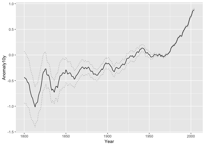
geom_ribbon画置信区间

clim <- subset(climate, Source == "Berkeley",
                 select=c("Year", "Anomaly10y", "Unc10y"))
clim %>% head()

##   Year Anomaly10y Unc10y
## 1 1800     -0.435  0.505
## 2 1801     -0.453  0.493
## 3 1802     -0.460  0.486
## 4 1803     -0.493  0.489
## 5 1804     -0.536  0.483
## 6 1805     -0.541  0.475

ggplot(clim, aes(x=Year, y=Anomaly10y)) +
    geom_ribbon(aes(ymin=Anomaly10y-Unc10y, 
                    ymax=Anomaly10y+Unc10y),
                # 相当于算出来每个点的标准差Unc10y，
                # 这是最简单的画置信区间的方式了
                alpha=0.2) +
geom_line()

geom_line画置信区间

ggplot(clim, aes(x=Year, y=Anomaly10y)) +
        geom_line(aes(y=Anomaly10y-Unc10y), colour="grey50", linetype="dotted") +
        geom_line(aes(y=Anomaly10y+Unc10y), colour="grey50", linetype="dotted") +
        geom_line()

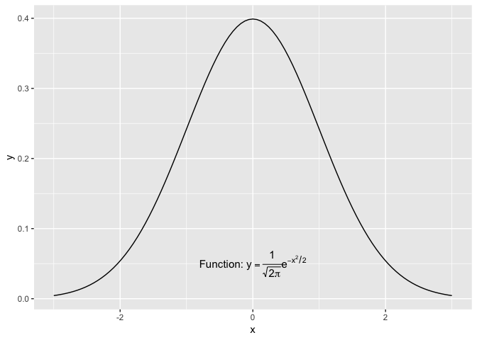
annotate图中加公式

不太懂的是这里的stat_function为什么能把c(-3,3)两个数画成一个表！

# A normal curve
p <- ggplot(data.frame(x=c(-3,3)), aes(x=x)) + 
  stat_function(fun = dnorm) 
p + annotate("text", x=2, y=0.3, parse=TRUE,
             label="frac(1, sqrt(2 * pi)) * e ^ {-x^2 / 2}")

p + annotate("text", x=0, y=0.05, parse=TRUE, size=4,
             label="'Function: ' * y==frac(1, sqrt(2*pi)) * e^{-x^2/2}")

pp. 180还可以加回归方程！

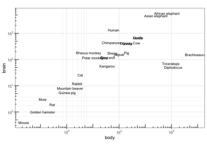
ggplot中(10^n)最好看的表达

library(MASS) # For the data set

## 
## Attaching package: 'MASS'

## The following object is masked from 'package:dplyr':
## 
##     select

library(scales) # For the trans and format functions

## 
## Attaching package: 'scales'

## The following object is masked from 'package:purrr':
## 
##     discard

## The following object is masked from 'package:readr':
## 
##     col_factor

ggplot(Animals, aes(x=body, y=brain, label=rownames(Animals))) + geom_text(size=3) +
annotation_logticks() +
scale_x_log10(breaks = trans_breaks("log10", function(x) 10^x),
                  labels = trans_format("log10", math_format(10^.x)),
minor_breaks = log10(5) + -2:5) + scale_y_log10(breaks = trans_breaks("log10", function(x) 10^x),
                  labels = trans_format("log10", math_format(10^.x)),
                  minor_breaks = log10(5) + -1:3) +
    coord_fixed() +
theme_bw()

## Warning in self$trans$transform(self$minor_breaks): 产生了NaNs

## Warning in self$trans$transform(self$minor_breaks): 产生了NaNs

scale_colour_brewer_example

stat_function举例函数图像

data_frame(x = c(-10,10)) %>% 
  ggplot(aes(x = x)) +
    stat_function(fun = function(x){1/(1+exp(-x))}
                  ) +
  labs(
    x = TeX("$z = \\ln(\\frac{p}{1-p})$"),
    y = TeX("$p = \\frac{1}{1 + e^{-z}}$")
  )

## Warning: `data_frame()` is deprecated, use `tibble()`.
## This warning is displayed once per session.

ggplot加入latex

使用 @Meschiari2015 的函数包latex2exp，所有的\改为\\，并使用TeX函数。 这是一个作者的教程。