概率图模型

0.1 PGM Daphne Koller

0.1.1 distribution

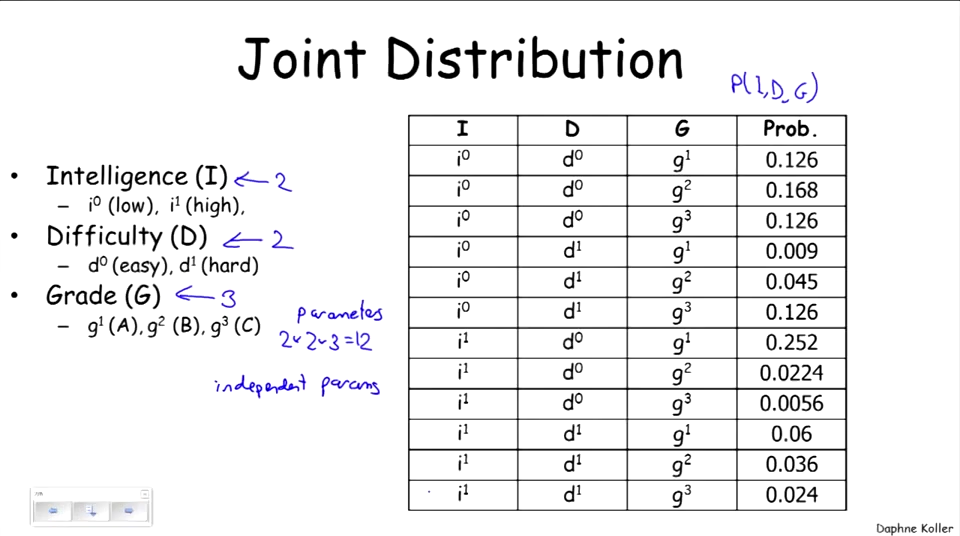
$conditioning是基于joint distribution完成的，例如condition on $g^1$，那么就只保留$g^1$的情况。$

Figure 1: conditioning是基于joint distribution完成的，例如condition on $g^1$，那么就只保留$g^1$的情况。

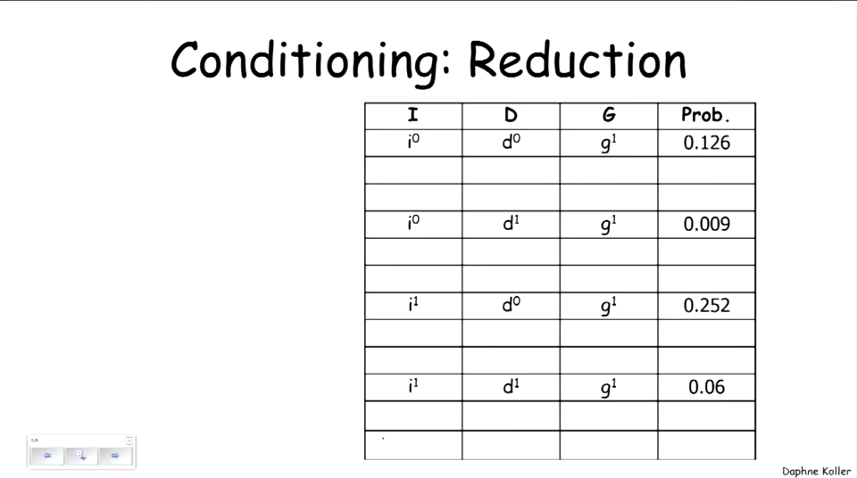
Figure 2: conditioning最关键的就是renormalization，这一步实现了joint distribution向conditioning的转化。

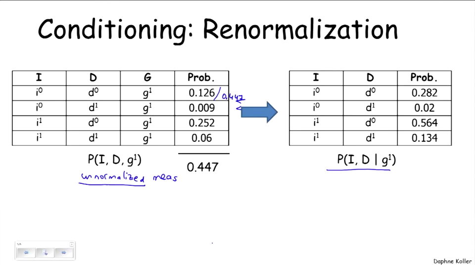
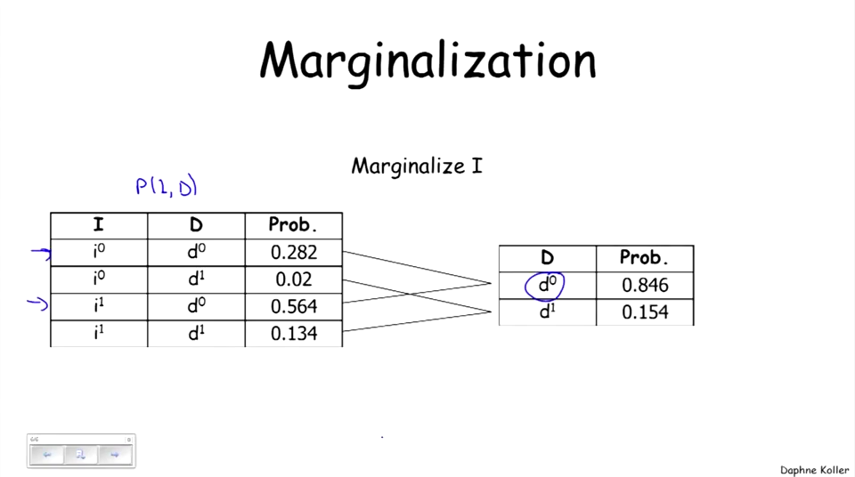
Figure 3: marginalizing的过程实际上是单变量distribution的思维，就是求和分布，这里常见于卡方检验。

0.1.2 factors

factors和之前distribution的内容很像，但是还是很有启发的。

这里的conditioning，就把I,D的情况全部列举了。

这个factor peoduct颇有join的感觉，非常好。

这里的factor marginalization和前面的marginalizing很像。

这个就是conditioning。

0.1.3 Bayesian Network Fundamentals

被箭头指向的展示条件概率分布，有向图表示因果判断。

联合分布的展示，就是所有节点概率相成。 $P(D),P(I),P(G)$之间相关，而不能直接用靠独立性假设而chain rule写入，

\[\times P(D,I,G) = P(D)\cdot P(I)\cdot P(G)\]

$P(G|I,D)$很好的处理了处理了这个问题，可以直接chain rule写入。

\[P(D,I,G) = P(D)\cdot P(I)\cdot P(G|I,D)\]

因此我们直接使用chain rule将概率相乘。

acyclic区别于马尔可夫链，not cyclic的意思。

这段证明非常有sense，任何联合分布，都可以用chain rule表示。

0.1.4 Reasoning Patterns

这是理解为什么贝叶斯的conditioning，和sense相同。

$P(d^1)\to P(d^1|g^3)$因为，grade 3的学生，上课的难概率肯定高。
$P(i^1)\to P(i^1|g^3)$因为，grade 3的学生，智商高的概率低。
$P(i^1|g^3)\to P(i^1|g^3,d^1)$因为，在grade 3的学生中，上的课难，智商高的概率高。

\[P(X_1 = 1 | Y = 1) = \frac{2}{3}\] \[P(X_2 = 1 | Y = 1) = \frac{2}{3}\] \[P(X_1 = 0 | Y = 1) = \frac{1}{3}\] \[P(X_2 = 0 | Y = 1) = \frac{1}{3}\]

$Y = 1$作为conditioning条件，把$Y \neq 1$的样本划掉。

\[P(X_2 = 1|Y = 1, X_1 = 1) = \frac{1}{2}\]

SAT拿到A的，理论上智商高。

0.1.5 Flow of Probabilistic Influence

这里讲的不是真正的因果关系，而是changes in believing，改变预期的概率，要看是否建立了x和y之间的cor。

\[\text{Difficulty} \to \text{Grade}\]

condition on Difficulty, changes believes about Grade. (???)

显然这里是负相关的¹。

\[\text{Grade} \gets \text{Intelligence} \to \text{SAT}\]

Grade的概率是会间接影响SAT的概率。

\[\text{V structure: } \text{Difficulty} \to \text{Grade} \gets \text{Intelligence}\]

这里没有推论，因为不能用一节课的难易来直观的推测学生的智商。

\[\text{Grade} \in Z: \times \text{Difficulty} \to \text{Grade} \to \text{Letter}\]

因为如果已知Grade了，那么能不能拿到Letter，完全由Grade决定，这个时候再提Difficulty，也没有什么影响了，除非我们在未知Grade的情况下，我们可以猜， Difficulty高，所以很可能Grade低，所以Letter拿不到。

\[\text{Grade} \in Z: \text{Difficulty} \to \text{Grade} \gets \text{Intelligence}\]

假设Grade很高，Difficulty大的，显然Intelligence高。同理，

\[\text{Grade} \in Z: \text{Difficulty} \to \text{Letter} \gets \text{Intelligence}\]

假设Letter好，Difficulty大的，显然Intelligence高。

下面说一个例子。

I is obs $\times$
I is not obs, nothing else $\times$
I is not obs, G is obs OK
I is not obs, G is not obs, L is obs OK

Active Trails的定义

已知任何V结构和其后代的信息时，
未知非V结构的节点的信息

0.1.6 Conditional Independence

\[\begin{alignat}{2} P(X,Y) &= P(X|Y)P(Y)\\ &\xrightarrow{X\perp Y}P(X|Y) = P(X)\\ &=P(X)P(Y)\\ P(X,Y) =P(X)P(Y) &:X\perp Y \end{alignat}\]

这个可以通过marginalization来查看。

可以先conditioning，再marginalizing来查看。

0.1.7 Independencies in Bayesian Networks

non-descendant，
i-maps
这两个知识点都没有看懂。

0.2 HMM

机器学习最重要的任务，是根据一些已观察到的证据(例如训练样本)来对感兴趣的未知变量(例如类别标记)进行估计和推测. 概率模型(probabilistic model)提供了一种描述框架, 将学习任务归结于计算变量的概率分布. 在概率模型中, 利用已知变量推测未知变量的分布称为“推断”(inference)，其核心是如何基于可观测变量推测出未知变量的条件分布.

具体来说，假定所关心的变量集合为 Y，可观测变量集合为’ O, 其他变量的集合为 $R,$ “生成式”(generative)模型考虑联合分布 $P(Y, R, O),$ “判别式” (discriminative)模型考虑条件分布 $P(Y, R \mid O) .$ 给定一组观测变量值, 推断就是要由 $P(Y, R, O)$ 或 $P(Y, R \mid O)$ 得到条件概率分布 $P(Y \mid O) .$

所以其他变量集合 R 只是放入，但是不参与推断。

概率图模型(probabilistic graphical model)是一类用图来表达变量相关关系的概率模型. 它以图为表示工具, 最常见的是用一个结点表示一个或一组随机变量, 结点之间的边表示变量间的概率相关关系, 即“变量关系图”。根据边的性质不同, 概率图模型可大致分为两类:

所以是否存在有向，就已经决定了是否需要判断因果关系。

第一类是使用有向无环图表示变量间的依赖关系, 称为有向图模型或贝叶斯网(Bayesian network);

所以贝叶斯常用于经济里面的因果推断。

第二类是使用无向图表示变量间的相关关系, 称为无向图模型或马尔可夫网 (Markov network).

HMM是不作为因果判断的。

隐马尔可夫模型(Hidden Markov Model, 简称 HMM)是结构最简单的动态贝叶斯网(dynamic Bayesian network), 这是一种著名的有向图模型, 主要用于时序数据建模, 在语音识别、自然语言处理等领域有广泛应用.

但是 HMM 是有向的，是有因果判断的。

0.2.1 结构信息

如图 14.1 所示, 隐马尔可夫模型中的变量可分为两组. 第一组是状态变量 $\left\{y_{1}, y_{2}, \ldots, y_{n}\right\},$ 其中 $y_{i} \in \mathcal{Y}$ 表示第 $i$ 时刻的系统状态. 通常假定状态变量是隐第二组是观测变量 $\left\{x_{1}, x_{2}, \ldots, x_{n}\right\},$ 其中 $x_{i} \in \mathcal{X}$ 表示第 $i$ 时刻的观测值.在隐马尔可夫模型中, 系统通常在多个状态 $\left\{s_{1}, s_{2}, \ldots, s_{N}\right\}$ 之间转换, 因此状态变量 $y_{i}$ 的取值观测变量 $x_{i}$ 可以是离散型也可以是连续型, 为便于讨论, 我们仅考虑离散型观测变量, 并假定其取值范围 $\mathcal{X}$ 为 $\left\{o_{1}, o_{2}, \ldots, o_{M}\right\}$

HMM 中的 y 是不可观测的，假设的，常常是监督学习里面的因变量。

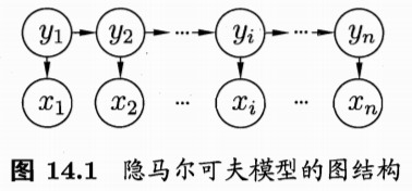
Figure 4: HMM 概率图结构。

图14.1 中的箭头表示了变量间的依赖关系. 在任一时刻, 观测变量的取值仅依赖于状态变量, 即 $x_{t}$ 由 $y_{t}$ 确定, 与其他状态变量及观测变量的取值无关.

因此这里是 $x \sim y$，虽然 y 才是因变量，类似于 SEM 里面 y 的定义。

同时, $t$ 时刻的状态 $y_{t}$ 仅依赖于 $t-1$ 时刻的状态 $y_{t-1},$ 与其余 $n-2$ 个状态无关.

单阶。

这就是所谓的“马尔可夫链”(Markov chain), 即: 系统下一时刻的状态仅由当前状态决定, 不依赖于以往的任何状态. 基于这种依赖关系, 所有变量的联合概率分布为

马尔科夫链的定义。

\[ P\left(x_{1}, y_{1}, \ldots, x_{n}, y_{n}\right)=P\left(y_{1}\right) P\left(x_{1} \mid y_{1}\right) \prod_{i=2}^{n} P\left(y_{i} \mid y_{i-1}\right) P\left(x_{i} \mid y_{i}\right) \]

显然每个单元的结构为 $x_i \sim y_i \sim y_{i-1}$，因此产生了 $P\left(y_{i} \mid y_{i-1}\right) P\left(x_{i} \mid y_{i}\right)$

因此这两个相乘的部分，可以分别定义。

0.2.2 三组参数

除了结构信息，欲确定一个隐马尔可夫模型还需以下三组参数:

状态转移概率: 模型在各个状态间转换的概率，通常记为矩阵 A = $\left[a_{i j}\right]_{N \times N},$ 其中

\[ a_{i j}=P\left(y_{t+1}=s_{j} \mid y_{t}=s_{i}\right), \quad 1 \leqslant i, j \leqslant N \]

表示在任意时刻 $t,$ 若状态为 $s_{i},$ 则在下一时刻状态为 $s_{j}$ 的概率.

主要定义$y_i \sim y_{i-1}$的关系。

输出观测概率: 模型根据当前状态获得各个观测值的概率, 通常记为矩阵 $\mathbf{B}=\left[b_{i j}\right]_{N \times M},$ 其中

\[ b_{i j}=P\left(x_{t}=o_{j} \mid y_{t}=s_{i}\right), \quad 1 \leqslant i \leqslant N, 1 \leqslant j \leqslant M \]

表示在任意时刻 $t,$ 若状态为 $s_{i},$ 则观测值 $o_{j}$ 被获取的概率.

主要定义$x_i \sim y_i$的关系。

初始状态概率: 模型在初始时刻各状态出现的概率，通常记为 = $\left(\pi_{1}, \pi_{2}, \ldots, \pi_{N}\right),$ 其中

\[ \pi_{i}=P\left(y_{1}=s_{i}\right), \quad 1 \leqslant i \leqslant N \]

表示模型的初始状态为 $s_{i}$ 的概率.

即$P\left(y_{1}\right) P\left(x_{1} \mid y_{1}\right)$

0.2.3 学习和推断

通过指定状态空间 Y、观测空间 X 和上述三组参数, 就能确定一个隐马尔可夫模型, 通常用其参数 $\lambda=[\mathbf{A}, \mathbf{B}, \pi]$ 来指代. 给定隐马尔可夫模型 $\lambda,$ 它按如下过程产生观测序列 $\left\{x_{1}, x_{2}, \ldots, x_{n}\right\}$

$\lambda=[\mathbf{A}, \mathbf{B}, \pi]$是三组参数集合。

设置 $t=1,$ 并根据初始状态概率 $\pi$ 选择初始状态 $y_{1}$

根据状态 $y_{t}$ 和输出观测概率 B 选择观況变量取值 $x_{t}$

根据状态 $y_{t}$ 和状态转移矩阵 A 特移模型状态, 即确定 $y_{t+1}$

若 $t<n,$ 设置 $t=t+1,$ 并转到第 (2) 步, 否则停止.

其中 $y_{t} \in\left\{s_{1}, s_{2}, \ldots, s_{N}\right\}$ 和 $x_{t} \in\left\{o_{1}, o_{2}, \ldots, o_{M}\right\}$ 分别为第 $t$ 时刻的状态和观测值.

状态不可测。

在实际应用中，人们常关注隐马尔可夫模型的三个基本问題：

$\left\{x_{1}, x_{2}, \ldots, x_{n}\right\}$ 的概率 $P(\mathbf{x} \mid \lambda) ?$ 换言之，如何评估模型与观测序列之启的匹配程度?

$\lambda$ 其实就是模型了，参与推断。

给定模型 $\lambda=[\mathbf{A}, \mathbf{B}, \pi]$ 和观测序列 $\mathbf{x}=\left\{x_{1}, x_{2}, \ldots, x_{n}\right\},$ 如何找到与此观测序列最匹配的状态序列 $\mathbf{y}=\left\{y_{1}, y_{2}, \ldots, y_{n}\right\}$ ? 换言之，如但根据观洛序列推断出隐藏的模型状态?

给定观测序列 $\mathbf{x}=\left\{x_{1}, x_{2}, \ldots, x_{n}\right\},$ 如何调整棋型参数 $\lambda=[\mathbf{A}, \mathbf{B}, \pi]$ 使得该序列出现的概率 $P(\mathbf{x} \mid \lambda)$ 最大? 换音之，如何训练模型使其舱最好地描述观测数据?

这三个问题其实都是和模型的估计方式、损失函数选择有关。

上述问題在现实应用中非常重要. 例如许多任务需根据以往的观測序列 $\left\{x_{1}, x_{2}, \ldots, x_{n-1}\right\}$ 来推断当前时刻最有可能的观测值 $x_{n},$ 这显然可转化为求取概率 $P(\mathbf{x} \mid$ 入)，即上述第一个问题;

逻辑类似于 RNN。

在语音识别等任务中, 观测值为语音信号, 隐藏状态为文字, 目标就是根据观测信号来推断最有可能的状态序列(即对应的文字)，即上述第二个问題;

这里地方不是很明白，Y 是不可观测的，为什么可以给一个显性的文字放在这里呢？
确定下这里是否是 Y 是文字，是需要推断的，然后 X 是语音，是一个监督任务？

在大多数现实应用中，人工指定模型参数已变得越来越不可行, 如何根据训练样本学得最优的模型参数, 恰是上述第三个问壓. 值得庆幸的是, 基于式(14.1)的条件独立性, 隐马尔可夫模型的这三个问題均能被高效求解。

0.3 MRF

马尔可夫随机场(Markov Random Field, 简称 MRF)是典型的马尔可夫网, 这是一种著名的无向图模型。图中每个结点表示一个或一组变量, 结点之间的边表示两个变量之间的依赖关系. 马尔可夫随机场有一组势函数(potential functions), 亦称“因子”(factor), 这是定义在变量子集上的非负实函数, 主要用于定义概率分布函数.

因为是无向图，所以是相关关系度量，非因果关系。

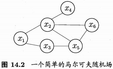
Figure 5: MRF 的简单结构。

图14.2 显示出一个简单的马尔可夫随机场. 对于图中结点的一个子集, 若其中任意两结点间都有边连接, 则称该结点子集为一个“团”(clique). 若在一个团中加入另外任何一个结点都不再形成团, 则称该团为“极大团”(maximal clique);

其中任意两结点间都有边连接，是一个极强的条件，和 DBSCAN 中对于核心点的定义很类似。

换言之, 极大团就是不能被其他团所包含的团. 例如，在图 14.2 中, $\left\{x_{1}, x_{2}\right\},\left\{x_{1}, x_{3}\right\},\left\{x_{2}, x_{4}\right\},\left\{x_{2}, x_{5}\right\},\left\{x_{2}, x_{6}\right\},\left\{x_{3}, x_{5}\right\},\left\{x_{5}, x_{6}\right\}$ 和 $\left\{x_{2}, x_{5}, x_{6}\right\}$ 都是团, 并且除了 $\left\{x_{2}, x_{5}\right\},\left\{x_{2}, x_{6}\right\}$ 和 $\left\{x_{5}, x_{6}\right\}$ 之外都是极大团 $;$ 但是, 因为 $x_{2}$ 和 $x_{3}$ 之间缺乏连接, $\left\{x_{1}, x_{2}, x_{3}\right\}$ 并不构成团. 显然, 每个结点至少出现在一个极大团中.

$\left\{x_{2}, x_{5}\right\},\left\{x_{2}, x_{6}\right\}$ 和 $\left\{x_{5}, x_{6}\right\}$ 加入其他的节点，还可以成团，比如$\left\{x_{2}, x_{5}\right\}$加入$x_6$可以成团。

在马尔可夫随机场中，多个变量之间的联合概率分布能基于团分解为多个因子的乘积，每个因子仅与一个团相关.

以团为一个单位，判断多因子之间的联合分布。

具体来说，对于 n 个变量 $\mathbf{x}=\left\{x_{1}, x_{2}, \ldots, x_{n}\right\},$ 所有团构成的集合为 $\mathcal{C},$ 与团 $Q \in \mathcal{C}$ 对应的变量集合记为 $\mathbf{x}_{Q},$ 则联合概率 $P(\mathbf{x})$ 定义为

这部分公式并不好理解

\[ P(\mathbf{x})=\frac{1}{Z} \prod_{Q \in \mathcal{C}} \psi_{Q}\left(\mathbf{x}_{Q}\right) \]

其中 $\psi_{Q}$ 为与团 Q 对应的势函数, 用于对团 Q 中的变量关系进行建模, $Z = \sum_{\mathbf{x}} \prod_{Q \in \mathcal{C}} \psi_{Q}\left(\mathbf{x}_{Q}\right)$ 为规范化因子，以确保 $P(\mathbf{x})$ 是被正确定义的概率. 在实际应用中, 精确计算 Z 通常很困难, 但许多任务往往并不需获得 Z 的精确值.

所以以一个极大团作为一个单位，进行联合分布估计。

显然, 若变量个数较多, 则团的数目将会很多(例如, 所有相互连接的两个变量都会构成团), 这就意味着式(14.2)会有很多乘积项，显然会给计算带来负担. 注意到若团 Q 不是极大团, 则它必被一个极大团 $Q^{*}$ 所包含, 即 $\mathbf{x}_{Q} \subseteq \mathbf{x}_{Q^{*}}$ 这意味着变量 x Q 之间的关系不仅体现在势函数 $\psi_{Q}$ 中, 还体现在 $\psi_{Q^{*}}$ 中. 于是, 联合概率 $P(\mathbf{x})$ 可基于极大团来定义. 假定所有极大团构成的集合为 $\mathcal{C}^{*},$ 则有

\[ P(\mathbf{x})=\frac{1}{Z^{*}} \prod_{Q \in \mathcal{C}^{*}} \psi_{Q}\left(\mathbf{x}_{Q}\right) \]

其中 $Z^{*}=\sum_{\mathbf{x}} \prod_{Q \in \mathcal{C}^{*}} \psi_{Q}\left(\mathbf{x}_{Q}\right)$ 为规范化因子. 例如图 14.2 中 $\mathbf{x}=\left\{x_{1}, x_{2}, \ldots,\right.$ $\left.x_{6}\right\},$ 联合概率分布 $P(\mathbf{x})$ 定义为

如图 5 基于极大团定义联合分布。

x1-x2
x1-x3
x2-x4
x2-x5-x6
x3-x5

\[ P(\mathbf{x})=\frac{1}{Z} \psi_{12}\left(x_{1}, x_{2}\right) \psi_{13}\left(x_{1}, x_{3}\right) \psi_{24}\left(x_{2}, x_{4}\right) \psi_{35}\left(x_{3}, x_{5}\right) \psi_{256}\left(x_{2}, x_{5}, x_{6}\right) \]

其中, 势函数 $\psi_{256}\left(x_{2}, x_{5}, x_{6}\right)$ 定义在极大团 $\left\{x_{2}, x_{5}, x_{6}\right\}$ 上, 由于它的存在, 使我们不再需为团 $\left\{x_{2}, x_{5}\right\},\left\{x_{2}, x_{6}\right\}$ 和 $\left\{x_{5}, x_{6}\right\}$ 构建势函数.

极大团包含了 $\left\{x_{2}, x_{5}\right\},\left\{x_{2}, x_{6}\right\}$ 和 $\left\{x_{5}, x_{6}\right\}$

在马尔可夫随机场中如何得到“条件独立性”呢?同样借助“分离”的概念, 如图 14.3 所示, 若从结点集 A 中的结点到 B 中的结点都必须经过结点集 $C$ 中的结点, 则称结点集 $A$ 和 $B$ 被结点集 $C$ 分离, C 称为“分离集”(separating set). 对马尔可夫随机场, 有全局马尔可夫性”(global Markov property): 给定两个变量子集的分离集, 则这两个变量子集条件独立. 也就是说, 图 14.3 中若令 $A, B$ 和 $C$ 对应的变量集分别为 $\mathbf{x}_{A}, \mathbf{x}_{B}$ 和 $\mathbf{x}_{C},$ 则 $\mathbf{x}_{A}$ 和 $\mathbf{x}_{B}$ 在给定x $_{C}$ 的条件下独立, 记为 $\mathbf{x}_{A} \perp \mathbf{x}_{B} \mid \mathbf{x}_{C}$

MRF 的独立性是条件的。

下面我们做一个简单的验证. 为便于讨论, 我们令图 14.3 中的 $A, B$ 和 $C$ 分别对应单变量 $x_{A}, x_{B}$ 和 $x_{C},$ 于是图 14.3 简化为图 14.4.

因此 MRF可以表示成变量集合之间的相关关系。

$分离集合$C$的定义。$ $分离集合$C$的定义。$

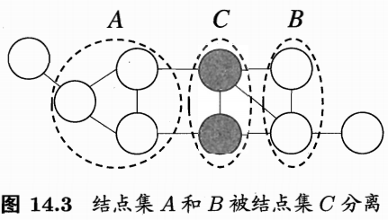
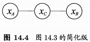
Figure 6: 分离集合$C$的定义。

基于条件概率的定义可得

\[ \begin{aligned} P\left(x_{A}, x_{B} \mid x_{C}\right) &=\frac{P\left(x_{A}, x_{B}, x_{C}\right)}{P\left(x_{C}\right)}=\frac{P\left(x_{A}, x_{B}, x_{C}\right)}{\sum_{x_{A}^{\prime}} \sum_{x_{B}^{\prime}} P\left(x_{A}^{\prime}, x_{B}^{\prime}, x_{C}\right)} \\ &=\frac{\frac{1}{Z} \psi_{A C}\left(x_{A}, x_{C}\right) \psi_{B C}\left(x_{B}, x_{C}\right)}{\sum_{x_{A}^{\prime}} \sum_{x_{B}^{\prime}} \frac{1}{Z} \psi_{A C}\left(x_{A}^{\prime}, x_{C}\right) \psi_{B C}\left(x_{B}^{\prime}, x_{C}\right)} \\ &=\frac{\psi_{A C}\left(x_{A}, x_{C}\right)}{\sum_{x_{A}^{\prime}} \psi_{A C}\left(x_{A}^{\prime}, x_{C}\right)} \cdot \frac{\psi_{B C}\left(x_{B}, x_{C}\right)}{\sum_{x_{B}^{\prime}} \psi_{B C}\left(x_{B}^{\prime}, x_{C}\right)} \end{aligned} \]

\[ \begin{aligned} P\left(x_{A} \mid x_{C}\right) &=\frac{P\left(x_{A}, x_{C}\right)}{P\left(x_{C}\right)}=\frac{\sum_{x_{B}^{\prime}} P\left(x_{A}, x_{B}^{\prime}, x_{C}\right)}{\sum_{x_{A}^{\prime}} \sum_{x_{B}^{\prime}} P\left(x_{A}^{\prime}, x_{B}^{\prime}, x_{C}\right)} \\ &=\frac{\sum_{x_{B}^{\prime}} \frac{1}{Z} \psi_{A C}\left(x_{A}, x_{C}\right) \psi_{B C}\left(x_{B}^{\prime}, x_{C}\right)}{\sum_{x_{A}^{\prime}} \sum_{x_{B}^{\prime}} \frac{1}{Z} \psi_{A C}\left(x_{A}^{\prime}, x_{C}\right) \psi_{B C}\left(x_{B}^{\prime}, x_{C}\right)} \\ &=\frac{\psi_{A C}\left(x_{A}, x_{C}\right)}{\sum_{x_{A}^{\prime}} \psi_{A C}\left(x_{A}^{\prime}, x_{C}\right)} \end{aligned} \]

由式(14.5)和(14.6)可知

公式比较复杂，不进行讨论。

\[ P\left(x_{A}, x_{B} \mid x_{C}\right)=P\left(x_{A} \mid x_{C}\right) P\left(x_{B} \mid x_{C}\right) \]

即 $x_{A}$ 和 $x_{B}$ 在给定 $x_{C}$ 时条件独立.

有这个推论即可。

由全局马尔可夫性可得到两个很有用的推论:

局部马尔可夫性(local Markov property): 给定某变量的邻接变量，则该变量条件独立于其他变量. 形式化地说, 令 V 为图的结点集, $n(v)$ 为结点 $v$ 在图上的邻接结点, $n^{*}(v)=n(v) \cup\{v\},$ 有 $\mathbf{x}_{v} \perp \mathbf{x}_{V \backslash n^{*}(v)} \mid \mathbf{x}_{n(v)}$

成对马尔可夫性(pairwise Markov property): 给定所有其他变量, 两个非邻接变量条件独立. 形式化地说，令图的结点集和边集分别为 V 和 $E,$ 对图中的两个结点 $u$ 和 $v,$ 若 $\langle u, v\rangle \notin E,$ 则 $\mathbf{x}_{u} \perp \mathbf{x}_{v} \mid \mathbf{x}_{V \backslash\langle u, v\rangle}$.

某变量的所有邻接变量组成的集合称为该变量的马尔可夫结”(Markov blanket).

现在我们来考察马尔可夫随机场中的势函数。显然，势函数 $\psi_{Q}\left(\mathbf{x}_{Q}\right)$ 的作用是定量刻画变量集 $\mathbf{x}_{Q}$ 中变量之间的相关关系，它应该是非负函数，且在所偏好的变量取值上有较大函数值. 例如，假定图 14.4 中的变量均为二值变量, 若势函数为

\[ \begin{array}{l} \psi_{A C}\left(x_{A}, x_{C}\right)=\left\{\begin{array}{ll} 1.5, & \text { if } x_{A}=x_{C} \\ 0.1, & \text { otherwise } \end{array}\right. \\ \psi_{B C}\left(x_{B}, x_{C}\right)=\left\{\begin{array}{ll} 0.2, & \text { if } x_{B}=x_{C} \\ 1.3, & \text { otherwise } \end{array}\right. \end{array} \]

则说明该模型偏好变量 $x_{A}$ 与 $x_{C}$ 据有相同的取值, $x_{B}$ 与 $x_{C}$ 据有不同的取值; 换言之, 在该模型中 $x_{A}$ 与 $x_{C}$ 正相关, $x_{B}$ 与 $x_{C}$ 负相关. 结合式(14.2)易知，令 $x_{A}$ 与 $x_{C}$ 相同且 $x_{B}$ 与 $x_{C}$ 不同的变量值指派将取得较高的联合概率. 为了满足非负性, 指数函数常被用于定义势函数, 即

\[ \psi_{Q}\left(\mathbf{x}_{Q}\right)=e^{-H_{Q}\left(\mathbf{x}_{Q}\right)} \]

$H_{Q}\left(\mathbf{x}_{Q}\right)$ 是一个定义在变量 $\mathbf{x}_{Q}$ 上的实值函数，常见形式为

\[ H_{Q}\left(\mathbf{x}_{Q}\right)=\sum_{u, v \in Q, u \neq v} \alpha_{u v} x_{u} x_{v}+\sum_{v \in Q} \beta_{v} x_{v} \]

其中 $\alpha_{u v}$ 和 $\beta_{v}$ 是参数. 上式中的第二项仅考虑单结点, 第一项则考虑每一对结点的关系.

这里只要抓住$\psi_{Q}$是非负的即可。

0.4 条件随机场

条件随机场可看作给定观测值的马尔可夫随机场，

如何理解给定观测值的马尔可夫随机场

也可看作对率回归的扩展对率回归参见3.3节

逻辑回归+传导。

条件随机场试图对多个变量在给定观测值后的条件概率进行建模。具体来说, 若令 $\mathbf{x}=\left\{x_{1}, x_{2}, \ldots, x_{n}\right\}$ 为观测序列, $\mathbf{y}=\left\{y_{1}, y_{2}, \ldots, y_{n}\right\}$ 为与之相应的标记序列, 则条件随机场的目标是构建条件概率模型 $P(\mathbf{y} \mid \mathbf{x}) .$ 需注意的是, 标记变量 y 可以是结构型变量, 即其分量之间具有某种相关性. 例如在自然语言处理的词性标注任务中, 观测数据为语句(即单词序列), 标记为相应的词性序列，具有线性序列结构, 如图 14.5(a)所示; 在语法分析任务中, 输出标记则是语法树，具有树形结构, 如图 14.5(b)所示。

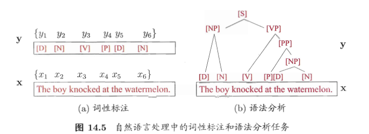
Figure 7: 语法树较少接触。

理论上来说，图 G 可具有任意结构，只要能表示标记变量之间的条件独立性关系即可. 但在现实应用中, 尤其是对标记序列建模时, 最常用的仍是图 14.6 所示的链式结构，即“链式条件随机场”(chain-structured CRF)。下面我们主要讨论这种条件随机场。

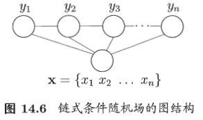
Figure 8: 和 Lafferty, McCallum, and Pereira (2001) 结构图不一样，但是差异也不大。

chain-structure CRF 我印象中也提到过

序列特征可以用 HMM、MRF、CRF 都可以。

与马尔可夫随机场定义联合概率的方式类似, 条件随机场使用势函数和图结构上的团来定义条件概率 P(y | x). 给定观测序列 x, 图 14.6 所示的链式条件随机场主要包含两种关于标记变量的团, 即单个标记变量 $\left\{y_{i}\right\}$ 以及相邻的标记变量 $\left\{y_{i-1}, y_{i}\right\} .$ 选择合适的势函数, 即可得到形如式(14.2)的条件概率定义. 在条件随机场中, 通过选用指数势函数并引入特征函数(feature function), 条件概率被定义为

这里注意的是也是度量 $\left\{y_{i-1}, y_{i}\right\} .$ 之间的相邻关系。

\[ P(\mathbf{y} \mid \mathbf{x})=\frac{1}{Z} \exp \left(\sum_{j} \sum_{i=1}^{n-1} \lambda_{j} t_{j}\left(y_{i+1}, y_{i}, \mathbf{x}, i\right)+\sum_{k} \sum_{i=1}^{n} \mu_{k} s_{k}\left(y_{i}, \mathbf{x}, i\right)\right) \]

其中 $t_{j}\left(y_{i+1}, y_{i}, \mathbf{x}, i\right)$ 是定义在观测序列的两个相邻标记位置上的转移特征函数(transition feature function), 用于刻画相邻标记变量之间的相关关系以及观测序列对它们的影响,

$t_{j}\left(y_{i+1}, y_{i}, \mathbf{x}, i\right)$ 相当于转换方程。

$s_{k}\left(y_{i}, \mathbf{x}, i\right)$ 是定义在观测序列的标记位置 $i$ 上的状态特征函数(status feature function), 用于刻画观测序列对标记变量的影响, $\lambda_{j}$ 和 $\mu_{k}$ 为参数, Z 为规范化因子, 用于确保式(14.11)是正确定义的概率. 显然, 要使用条件随机场, 还需定义合适的特征函数. 特征函数通常是实值函数, 以刻画数据的一些很可能成立或期望成立的经验特性. 以图 14.5(a) 的词性标注任务为例, 若采用转移特征函数

\[ t_{j}\left(y_{i+1}, y_{i}, \mathbf{x}, i\right)=\left\{\begin{array}{ll} 1, & \text { if } y_{i+1}=[P], y_{i}=[V] \text { and } x_{i}={ }^{4} \mathrm{knock}^{\prime \prime} \\ 0, & \text { otherwise } \end{array}\right. \]

则表示第 $i$ 个观测值 $x_{i}$ 为单词“knock”时, 相应的标记 $y_{i}$ 和 $y_{i+1}$ 很可能分别为 [V] 和 [P]. 若采用状态特征函数

\[ s_{k}\left(y_{i}, \mathbf{x}, i\right)=\left\{\begin{array}{ll} 1, & \text { if } y_{i}=[V] \text { and } x_{i}={ }^{\prime} \mathrm{knock}^{\prime \prime} \\ 0, & \text { otherwise } \end{array}\right. \]

则表示观测值 $x_{i}$ 为单词“knock”时, 它所对应的标记很可能为 [V]. 对比式(14.11)和(14.2)可看出, 条件随机场和马尔可夫随机场均使用团上的势函数定义概率, 两者在形式上没有显著区别; 但条件随机场处理的是条件概率, 而马尔可夫随机场处理的是联合概率.

因为 MRF 没有标签，所以度量的是联合分布，在这里需要求解$P(\mathbf{y} \mid \mathbf{x})$，所以是条件分布。

参考 Lafferty, McCallum, and Pereira (2001)

We present conditional random felds, a framework for building probabilistic models to segment and label sequence data.

分割、标注序列数据。

所以是否可以做文本分割？

Conditional random felds oﬀer several advantages over hidden Markov models and stochastic grammars for such tasks, including the ability to relax strong independence assumptions made in those models. Conditional random felds also avoid a fundamental limitation of maximum entropy Markov models (MEMMs) and other discriminative Markov models based on directed graphical models, which can be biased towards states with few successor states. We present iterative parameter estimation algorithms for conditional random felds and compare the performance of the resulting models to HMMs and MEMMs on synthetic and natural-language data.

CRF 比 HMM 等提高了对 NLP 数据的处理。

0.5 Introduction

The need to segment and label sequences arises in many different problems in several scientific fields. Hidden Markov models (HMMs) and stochastic grammars are well understood and widely used probabilistic models for such problems.

整个应用还是非常广泛的。

In computational biology, HMMs and stochastic grammars have been successfully used to align biological sequences, find sequences homologous to a known evolutionary family, and analyze RNA secondary structure (Durbin et al., 1998).

RNA 的序列，寻找频繁子序列。

In computational linguistics and computer science, HMMs and stochastic grammars have been applied to a wide variety of problems in text and speech processing, including topic segmentation, part-ofspeech (POS) tagging, information extraction, and syntactic disambiguation (Manning & Schütze, 1999).

主题分割、词性标注、信息抽取、语义识别。

HMMs and stochastic grammars are generative models, assigning a joint probability to paired observation and label sequences; the parameters are typically trained to maxi-mize the joint likelihood of training examples. To define a joint probability over observation and label sequences, a generative model needs to enumerate all possible observation sequences, typically requiring a representation in which observations are task-appropriate atomic entities, such as words or nucleotides. In particular, it is not practical to represent multiple interacting features or long-range dependencies of the observations, since the inference problem for such models is intractable.

作者论述 HMM 和 SG 都不能生成长序列。

This difficulty is one of the main motivations for looking at conditional models as an alternative.

前面都是生成式学习，现在是判别式，条件式学习。

A conditional model specifies the probabilities of possible label sequences given an observation sequence. Therefore, it does not expend modeling effort on the observations, which at test time are fixed anyway. Furthermore, the conditional probability of the label sequence can depend on arbitrary, nonindependent features of the observation sequence without forcing the model to account for the distribution of those dependencies. The chosen features may represent attributes at different levels of granularity of the same observations (for example, words and characters in English text), or aggregate properties of the observation sequence (for instance, text layout). The probability of a transition between labels may depend not only on the current observation, but also on past and future observations, if available. In contrast, generative models must make very strict independence assumptions on the observations, for instance conditional independence given the labels, to achieve tractability.

如 HMM，生成式学习假定变量之间是独立的，但是判别式学习可以更加宽松的假设。

Maximum entropy Markov models (MEMMs) are conditional probabilistic sequence models that attain all of the above advantages (McCallum et al., 2000). In MEMMs, each source state $^{1}$ has a exponential model that takes the observation features as input, and outputs a distribution over possible next states. These exponential models are trained by an appropriate iterative scaling method in the maximum entropy framework. Previously published experimental results show MEMMs increasing recall and doubling precision relative to HMMs in a FAQ segmentation task.

MEMMs 是条件概率序列模型，比 HMM 更好些。

MEMMs and other non-generative finite-state models based on next-state classifiers, such as discriminative Markov models (Bottou, 1991), share a weakness we call here the label bias problem: the transitions leaving a given state compete only against each other, rather than against all other transitions in the model. In probabilistic terms, transition scores are the conditional probabilities of possible next states given the current state and the observation sequence. This per-state normalization of transition scores implies a “conservation of score mass” (Bottou, 1991) whereby all the mass that arrives at a state must be distributed among the possible successor states. An observation can affect which destination states get the mass, but not how much total mass to pass on. This causes a bias toward states with fewer outgoing transitions. In the extreme case, a state with a single outgoing transition effectively ignores the observation. In those cases, unlike in HMMs, Viterbi decoding cannot downgrade a branch based on observations after the branch point, and models with statetransition structures that have sparsely connected chains of states are not properly handled. The Markovian assumptions in MEMMs and similar state-conditional models insulate decisions at one state from future decisions in a way that does not match the actual dependencies between consecutive states.

MEMMs 和 HMM 都有 label bias 的问题，但是没看懂为什么 HMM 也有？

This paper introduces conditional random fields (CRFs), a sequence modeling framework that has all the advantages of MEMMs but also solves the label bias problem in a principled way. The critical difference between CRFs and MEMMs is that a MEMM uses per-state exponential models for the conditional probabilities of next states given the current state, while a CRF has a single exponential model for the joint probability of the entire sequence of labels given the observation sequence. Therefore, the weights of different features at different states can be traded off against each other.

CRFs 和 MEMMS 都是序列模型，的唯一差异是解决了 lebal bias，也就是不仅仅是用当前状态预测下一个状态，而是用整个序列的联合分布去预测下一个状态。

We present the model, describe two training procedures and sketch a proof of convergence. We also give experimental results on synthetic data showing that CRFs solve the classical version of the label bias problem, and, more significantly, that CRFs perform better than HMMs and MEMMs when the true data distribution has higher-order dependencies than the model, as is often the case in practice.

当存在高阶相关性时，CRFs 比 HMM、MEMMs 更好，

Finally, we confirm these results as well as the claimed advantages of conditional models by evaluating HMMs, MEMMs and CRFs with identical state structure on a part-of-speech tagging task.

也解决了词性标注的问题。

CRFs jieba 有么？词性标注，或者北大的分词包

0.6 The Label Bias Problem

这是作者主要解决的问题。

Classical probabilistic automata (Paz, 1971), discriminative Markov models (Bottou, 1991), maximum entropy taggers (Ratnaparkhi, 1996), and MEMMs, as well as non-probabilistic sequence tagging and segmentation models with independently trained next-state classifiers (Punyakanok & Roth, 2001) are all potential victims of the label bias problem.

MEMMs 以前的模型都存在这个问题。

For example, Figure 1 represents a simple finite-state model designed to distinguish between the two words rib and rob. Suppose that the observation sequence is $r$ i $b$. In the first time step, r matches both transitions from the start state, so the probability mass gets distributed roughly equally among those two transitions. Next we observe i. Both states 1 and 4 have only one outgoing transition. State 1 has seen this observation often in training, state 4 has almost never seen this observation; but like state $1,$ state 4 has no choice but to pass all its mass to its single outgoing transition, since it is not generating the observation, only conditioning on it. Thus, states with a single outgoing transition effectively ignore their observations. More generally, states with low-entropy next state distributions will take little notice of observations. Returning to the example, the top path and the bottom path will be about equally likely, independently of the observation sequence. If one of the two words is slightly more common in the training set, the transitions out of the start state will slightly prefer its corresponding transition, and that word’s state sequence will always win. This behavior is demonstrated experimentally in Section 5

这里提到的 always win 有什么问题么，正面这个例子还是没有看懂。

(ref:20200821100016-plot)

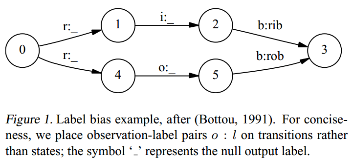
Figure 9: (ref:20200821100016-plot)

Léon Bottou (1991) discussed two solutions for the label bias problem.

One is to change the state-transition structure of the model. In the above example we could collapse states 1 and $4,$ and delay the branching until we get a discriminating observation. This operation is a special case of determinization (Mohri, 1997), but determinization of weighted finite-state machines is not always possible, and even when possible, it may lead to combinatorial explosion.

似乎是强行把状态1和4全局的看。

The other solution mentioned is to start with a fullyconnected model and let the training procedure figure out a good structure. But that would preclude the use of prior structural knowledge that has proven so valuable in information extraction tasks (Freitag & McCallum, 2000).

全连接，用模型去训练？

Proper solutions require models that account for whole state sequences at once by letting some transitions “vote” more strongly than others depending on the corresponding observations. This implies that score mass will not be conserved, but instead individual transitions can “amplify” or “dampen” the mass they receive. In the above example, the transitions from the start state would have a very weak effect on path score, while the transitions from states 1 and 4 would have much stronger effects, amplifying or damping depending on the actual observation, and a proportionally higher contribution to the selection of the Viterbi path.3

作者想说明，state 1 和 4 才是路径中贡献最大的，应该进行调整。

In the related work section we discuss other heuristic model classes that account for state sequences globally rather than locally. To the best of our knowledge, CRFs are the only model class that does this in a purely probabilistic setting, with guaranteed global maximum likelihood convergence.

CRF 解决的就是全局最优化。

0.7 Conditional Random Fields

In what follows, $\mathbf{X}$ is a random variable over data sequences to be labeled, and $\mathbf{Y}$ is a random variable over corresponding label sequences. All components $\mathbf{Y}_{i}$ of $\mathbf{Y}$ are assumed to range over a finite label alphabet $\mathcal{Y} .$ For example, $\mathbf{X}$ might range over natural language sentences and $\mathbf{Y}$ range over part-of-speech taggings of those sentences, with $\mathcal{Y}$ the set of possible part-of-speech tags.

作者举了一个词性标注的例子。

The random variables $\mathbf{X}$ and $\mathbf{Y}$ are jointly distributed, but in a discriminative framework we construct a conditional model $p(\mathbf{Y} \mid \mathbf{X})$ from paired observation and label sequences, and do not explicitly model the marginal $p(\mathbf{X})$.

CRF 是一个判别式而非生成式的例子。

0.7.1 Definition.

Let $G=(V, E)$ be a graph such that $\mathbf{Y}=\left(\mathbf{Y}_{v}\right)_{v \in V},$ so that $\mathbf{Y}$ is indexed by the vertices of $G .$ Then $(\mathbf{X}, \mathbf{Y})$ is a conditional random field in case, when conditioned on $\mathbf{X}$, the random variables $\mathbf{Y}_{v}$ obey the Markov property with respect to the graph: $p\left(\mathbf{Y}_{v} \mid \mathbf{X}, \mathbf{Y}_{w}, w \neq v\right)=p\left(\mathbf{Y}_{v} \mid \mathbf{X}, \mathbf{Y}_{w}, w \sim v\right),$ where $w \sim v$ means that $w$ and $v$ are neighbors in $G .$

CRF的定义，虽然是判别式，但是 conditional on 所有其他变量$p\left(\mathbf{Y}_{v} \mid \mathbf{X}, \mathbf{Y}_{w}, w \neq v\right)$

Thus, a CRF is a random field globally conditioned on the observation $\mathbf{X}$. Throughout the paper we tacitly assume that the graph $G$ is fixed. In the simplest and most important example for modeling sequences, $G$ is a simple chain or line: $G=(V=\{1,2, \ldots m\}, E=\{(i, i+1)\})$ $\mathbf{X}$ may also have a natural graph structure; yet in general it is not necessary to assume that $\mathbf{X}$ and $\mathbf{Y}$ have the same graphical structure, or even that $\mathbf{X}$ has any graphical structure at all. However, in this paper we will be most concerned with sequences $\mathbf{X}=\left(\mathbf{X}_{1}, \mathbf{X}_{2}, \ldots, \mathbf{X}_{n}\right)$ and $\mathbf{Y}=\left(\mathbf{Y}_{1}, \mathbf{Y}_{2}, \ldots, \mathbf{Y}_{n}\right)$

作者的假设是 $\mathbf{Y}$ 和 $\mathbf{X}$ 是等长的，但是理论长度、结构都可以不一样。

也可以满足树结构。

If the graph $G=(V, E)$ of $\mathbf{Y}$ is a tree (of which a chain is the simplest example), its cliques are the edges and vertices. Therefore, by the fundamental theorem of random fields (Hammersley & Clifford, 1971), the joint distribution over the label sequence $\mathbf{Y}$ given $\mathbf{X}$ has the form

\[ \begin{array}{l} p_{\theta}(\mathbf{y} \mid \mathbf{x}) \propto \\ \exp \left(\sum_{e \in E, k} \lambda_{k} f_{k}\left(e,\left.\mathbf{y}\right|_{e}, \mathbf{x}\right)+\sum_{v \in V, k} \mu_{k} g_{k}\left(v,\left.\mathbf{y}\right|_{v}, \mathbf{x}\right)\right) \end{array} \]

where $x$ is a data sequence, $y$ a label sequence, and $\left.y\right|_{S}$ is the set of components of $y$ associated with the vertices in subgraph $S$. We assume that the features $f_{k}$ and $g_{k}$ are given and fixed. For example, a Boolean vertex feature $g_{k}$ might be true if the word $\mathbf{X}_{i}$ is upper case and the $\operatorname{tag} \mathbf{Y}_{i}$ is “proper noun.”

The parameter estimation problem is to determine the parameters $\theta=\left(\lambda_{1}, \lambda_{2}, \ldots ; \mu_{1}, \mu_{2}, \ldots\right)$ from training data $\mathcal{D}=\left\{\left(\mathbf{x}^{(i)}, \mathbf{y}^{(i)}\right)\right\}_{i=1}^{N}$ with empirical distribution $\tilde{p}(\mathbf{x}, \mathbf{y})$ In Section 4 we describe an iterative scaling algorithm that maximizes the log-likelihood objective function $\mathcal{O}(\theta)$ :

\[ \begin{aligned} \mathcal{O}(\theta) &=\sum_{i=1}^{N} \log p_{\theta}\left(\mathbf{y}^{(i)} \mid \mathbf{x}^{(i)}\right) \\ & \propto \sum_{\mathbf{x}, \mathbf{y}} \tilde{p}(\mathbf{x}, \mathbf{y}) \log p_{\theta}(\mathbf{y} \mid \mathbf{x}) \end{aligned} \]

As a particular case, we can construct an HMM-like CRF by defining one feature for each state pair $\left(y^{\prime}, y\right),$ and one feature for each state-observation pair $(y, x):$

\[ \begin{aligned} f_{y^{\prime}, y}(<u, v>, \mathbf{y} \mid<u, v>, \mathbf{x}) &=\delta\left(\mathbf{y}_{u}, y^{\prime}\right) \delta\left(\mathbf{y}_{v}, y\right) \\ g_{y, x}\left(v,\left.\mathbf{y}\right|_{v}, \mathbf{x}\right) &=\delta\left(\mathbf{y}_{v}, y\right) \delta\left(\mathbf{x}_{v}, x\right) \end{aligned} \]

The corresponding parameters $\lambda_{y^{\prime}, y}$ and $\mu_{y, x}$ play a similar role to the (logarithms of the) usual HMM parameters $p\left(y^{\prime} \mid y\right)$ and $p(x \mid y) .$ Boltzmann chain models (Saul & Jordan, 1996; MacKay, 1996) have a similar form but use a single normalization constant to yield a joint distribution, whereas CRFs use the observation-dependent normalization $Z(\mathbf{x})$ for conditional distributions. Although it encompasses HMM-like models, the class of conditional random fields is much more expressive, because it allows arbitrary dependencies on the observation sequence.

整体公式不方便理解，但是可以查看图像。

In addition, the features do not need to specify completely a state or observation, so one might expect that the model can be estimated from less training data. Another attractive property is the convexity of the loss function; indeed, CRFs share all of the convexity properties of general maximum entropy models.

因为 CRF 考虑了更多的连接，因此可以使用更少的训练样本。

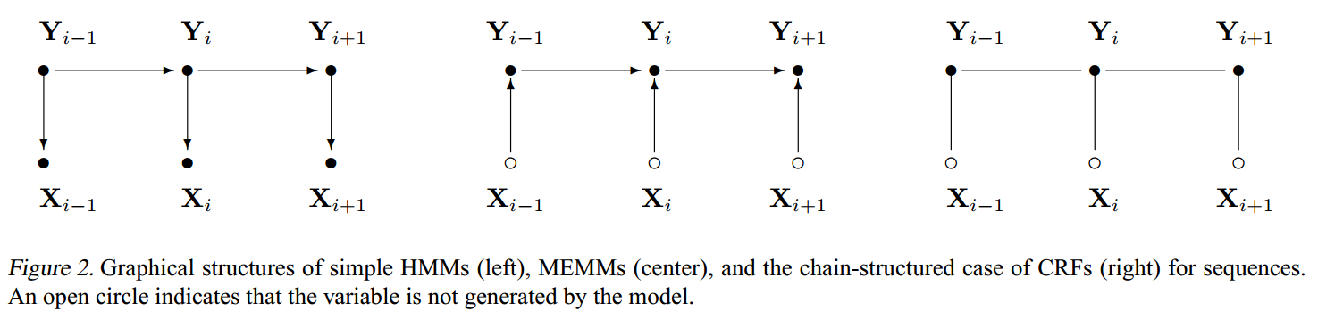
Figure 10: HMM、MEMM、CRF 的比较。

可以转换为一个矩阵结构。

For the remainder of the paper we assume that the dependencies of $\mathbf{Y},$ conditioned on $\mathbf{X},$ form a chain. To $\operatorname{sim}=$ plify some expressions, we add special start and stop states $\mathbf{Y}_{0}=$ start and $\mathbf{Y}_{n+1}=$ stop. Thus, we will be using the graphical structure shown in Figure $2 .$ For a chain structure, the conditional probability of a label sequence can be expressed concisely in matrix form, which will be useful in describing the parameter estimation and inference algorithms in Section 4. Suppose that $p_{\theta}(\mathbf{Y} \mid \mathbf{X})$ is a CRF given by (1). For cach position i in the observation sequence $\mathbf{x},$ we define the $|\mathcal{Y}| \times|\mathcal{Y}|$ matrix random variable

\[ \begin{array}{c} M_{i}(\mathbf{x})=\left[M_{i}\left(y^{\prime}, y \mid \mathbf{x}\right)\right] \text { by } \\ M_{i}\left(y^{\prime}, y \mid \mathbf{x}\right)=\exp \left(\Lambda_{i}\left(y^{\prime}, y \mid \mathbf{x}\right)\right) \\ \Lambda_{i}\left(y^{\prime}, y \mid \mathbf{x}\right)=\sum_{k} \lambda_{k} f_{k}\left(e_{i},\left.\mathbf{Y}\right|_{e_{i}}=\left(y^{\prime}, y\right), \mathbf{x}\right)+ \\ & \sum_{k} \mu_{k} g_{k}\left(v_{i},\left.\mathbf{Y}\right|_{v_{4}}=y, \mathbf{x}\right) \end{array} \]

where $e_{i}$ is the edge with labels $\left(\mathbf{Y}_{i-1}, \mathbf{Y}_{i}\right)$ and $v_{i}$ is the vertex with label $\mathbf{Y}_{i}$. In contrast to generative models, conditional models like CRFs do not need to enumerate over all possible observation sequences $\mathbf{x}$, and therefore these matrices can be computed directly as needed from a given training or test observation sequence $x$ and the paramcter vector $\theta$. Then the normalization (partition function) $Z_{\theta}(\mathbf{x})$ is the (start, stop) entry of the product of these matrices:

\[ Z_{\theta}(\mathbf{x})=\left(M_{1}(\mathbf{x}) M_{2}(\mathbf{x}) \cdots M_{n+1}(\mathbf{x})\right)_{\text {start,stop }} \]

Using this notation, the conditional probability of a label sequence $y$ is written as

\[ p_{\theta}(\mathbf{y} \mid \mathbf{x})=\frac{\prod_{i=1}^{n+1} M_{i}\left(\mathbf{y}_{i-1}, \mathbf{y}_{i} \mid \mathbf{x}\right)}{\left(\prod_{i=1}^{n+1} M_{i}(\mathbf{x})\right)_{\text {start, stop }}} \]

where $y_{0}=s t a r t$ and $y_{n+1}=s t o p$

0.8 Parameter Estimation for CRFs

很多推导都是比较少接触的，可以多看看

迭代方式是指数相乘的。

We now describe two iterative scaling algorithms to find the parameter vector $\theta$ that maximizes the log-likelihood of the training data. Both algorithms are based on the improved iterative scaling (IIS) algorithm of Della Pietra et al. (1997)$;$ the proof technique based on auxiliary functions can be extended to show convergence of the algorithms for CRFs. Iterative scaling algorithms update the weights as $\lambda_{k} \leftarrow$ $\lambda_{k}+\delta \lambda_{k}$ and $\mu_{k} \leftarrow \mu_{k}+\delta \mu_{k}$ for appropriately chosen $\delta \lambda_{k}$ and $\delta \mu_{k}$. In particular, the IIS update $\delta \lambda_{k}$ for an edge feature $f_{k}$ is the solution of

\[ \begin{array}{c} \tilde{E}\left[f_{k}\right] \stackrel{\text { def }}{=} \sum_{\mathbf{x}, \mathbf{y}} \tilde{p}(\mathbf{x}, \mathbf{y}) \sum_{i=1}^{n+1} f_{k}\left(e_{i},\left.\mathbf{y}\right|_{e_{i}}, \mathbf{x}\right) \\ =\sum_{\mathbf{x}, \mathbf{y}} \tilde{p}(\mathbf{x}) p(\mathbf{y} \mid \mathbf{x}) \sum_{i=1}^{n+1} f_{k}\left(e_{i},\left.\mathbf{y}\right|_{c_{i}}, \mathbf{x}\right) e^{\delta \lambda_{4} T(\mathbf{x}, \mathbf{y})} \end{array} \]

where $T(\mathbf{x}, \mathbf{y})$ is the total feature count

\[ T(\mathbf{x}, \mathbf{y}) \stackrel{\text { sf }}{=} \sum_{i, k} f_{k}\left(e_{i},\left.\mathbf{y}\right|_{c_{i}}, \mathbf{x}\right)+\sum_{i, k} g_{k}\left(v_{i},\left.\mathbf{y}\right|_{v_{i}}, \mathbf{x}\right) \]

The equations for vertex feature updates $\delta \mu_{k}$ have similar form. However, efficiently computing the exponential sums on the right-hand sides of these equations is problematic, because $T(\mathbf{x}, \mathbf{y})$ is a global property of $(\mathbf{x}, \mathbf{y}),$ and dynamic programming will sum over sequences with potentially varying $T$. To deal with this, the first algorithm, Algorithm S, uses a “slack feature.” The second, Algorithm T, keeps track of partial $T$ totals. For Algorithm S, we define the slack feature by

\[ \begin{aligned} s(\mathbf{x}, \mathbf{y}) & \stackrel{\text { def }}{=} \\ S &-\sum_{i} \sum_{k} f_{k}\left(e_{i},\left.\mathbf{y}\right|_{e_{i}}, \mathbf{x}\right)-\sum_{i} \sum_{k} g_{k}\left(v_{i},\left.\mathbf{y}\right|_{v_{i}}, \mathbf{x}\right) \end{aligned} \]

where $S$ is a constant chosen so that $s\left(\mathbf{x}^{(i)}, \mathbf{y}\right) \geq 0$ for all $\mathbf{y}$ and all observation vectors $\mathbf{x}^{(i)}$ in the training set, thus making $T(\mathbf{x}, \mathbf{y})=S .$ Feature $s$ is “global,” that is, it does not correspond to any particular edge or vertex.

For each index $i=0, \ldots, n+1$ we now define the forward vectors $\alpha_{i}(\mathrm{x})$ with base case

\[ \alpha_{0}(y \mid \mathbf{x})=\left\{\begin{array}{ll} 1 & \text { if } y=\text { start } \\ 0 & \text { otherwise } \end{array}\right. \]

后面部分也不是特别看得懂。

0.9 Experiments

前面这一段实验的表述，需要掌握了第四部分会更加容易懂一点，文欣、武神也可以看看

0.9.1 Modeling label bias

0.9.2 Modeling mixed-order sources

0.9.3 POS tagging experiments

0.10 Further Aspects of CRFs

Conditional random fields can be trained using the exponential loss objective function used by the AdaBoost algorithm (Freund & Schapire, 1997). Typically, boosting is applied to classification problems with a small, fixed number of classes; applications of boosting to sequence labeling have treated each label as a separate classification problem (Abney et al., 1999). However, it is possible to apply the parallel update algorithm of Collins et al. (2000) to optimize the per-sequence exponential loss. This requires a forward-backward algorithm to compute efficiently certain feature expectations, along the lines of Algorithm $\mathrm{T},$ except that each feature requires a separate set of forward and backward accumulators.

CRF 可以和 AdaBoost 结合？

TrAdaBoost是由AdaBoost（Adaptive Boosting）算法演变而来的。 AdaBoost算法的基本思想是：当一个训练样本被错误分类时，算法就会认为这个样本是难分类的，就会适当地增加其样本权重，下次训练时这个样本被分错的概率就会降低。 (梅子行 2020)
CRF 可以和 XGBoost 结合么？

特征工程、DP相关

Another attractive aspect of CRFs is that one can implement efficient feature selection and feature induction al- gorithms for them. That is, rather than specifying in advance which features of $(\mathbf{X}, \mathbf{Y})$ to use, we could start from feature-generating rules and evaluate the benefit of generated features automatically on data. In particular, the feature induction algorithms presented in Della Pietra et al. (1997) can be adapted to fit the dynamic programming techniques of conditional random fields.

这里最好的举例说明，直接写ABC，不直观，难以懂。↩