Paper Review

李家翔

2020-11-06

1. 使用 RMarkdown 的 child 参数，进行文档拼接。
2. 这样拼接以后的笔记方便复习。
3. 相关问题提交到 Issue

1 Weight Decay

Recall that in our polynomial regression example (Section 4.4) we could limit our model’s capacity simply by tweaking the degree of the fitted polynomial. Indeed, limiting the number of features is a popular technique to mitigate overfitting. However, simply tossing aside features can be too blunt an instrument for the job. Sticking with the polynomial regression example, consider what might happen with high-dimensional inputs. The natural extensions of polynomials to multivariate data are called monomials, which are simply products of powers of variables. The degree of a monomial is the sum of the powers. For example, \(x_{1}^{2} x_{2},\) and \(x_{3} x_{5}^{2}\) are both monomials of degree 3.

引入概念 ‘monomial is the sum of the powers’。

Note that the number of terms with degree \(d\) blows up rapidly as \(d\) grows larger. Given \(k\) variables, the number of monomials of degree \(d\) (i.e., \(k\) multichoose \(d\) ) is \(\left(\begin{array}{c}k-1+d \\ k-1\end{array}\right)\). Even small changes in degree, say from 2 to 3, dramatically increase the complexity of our model. Thus we often need a more fine-grained tool for adjusting function complexity.

这个概念就是从 FM 等模型的角度上实现。

1.0.1 Norms and Weight Decay

We have described both the \(L_{2}\) norm and the \(L_{1}\) norm, which are special cases of the more general \(L_{p}\) norm in Section \(2.3 .10 .\) Weight decay (commonly called \(L_{2}\) regularization), might be the most widely-used technique for regularizing parametric machine learning models. The technique is motivated by the basic intuition that among all functions \(f\), the function \(f=0\) (assigning the value 0 to all inputs) is in some sense the simplest, and that we can measure the complexity of a function by its distance from zero. But how precisely should we measure the distance between a function and zero? There is no single right answer. In fact, entire branches of mathematics, including parts of functional analysis and the theory of Banach spaces, are devoted to answering this issue.

weight decay 就是 L2 正则化？ 是的，结束。

2 词向量以及训练

2.1 词向量

对于向量\(\boldsymbol{x}, \boldsymbol{y} \in \mathbb{R}^d\)，它们的余弦相似度是它们之间夹角的余弦值

\[\frac{\boldsymbol{x}^\top \boldsymbol{y}}{\|\boldsymbol{x}\| \|\boldsymbol{y}\|} \in [-1, 1].\]

由于任何两个不同词的one-hot向量的余弦相似度都为0，多个不同词之间的相似度难以通过one-hot向量准确地体现出来。

任意两个词的相关性都是0，这一步假设太不符合实际了，至少同义词就不符合这个假设。

2.1.1 跳字模型

跳字模型假设基于某个词来生成它在文本序列周围的词。举个例子，假设文本序列是“the”“man”“loves”“his”“son”。以“loves”作为中心词，设背景窗口大小为2。如图10.1所示，跳字模型所关心的是，给定中心词“loves”，生成与它距离不超过2个词的背景词“the”“man”“his”“son”的条件概率，即

\[P(\textrm{``the"},\textrm{``man"},\textrm{``his"},\textrm{``son"}\mid\textrm{``loves"}).\]

假设给定中心词的情况下，背景词的生成是相互独立的，那么上式可以改写成

\[P(\textrm{``the"}\mid\textrm{``loves"})\cdot P(\textrm{``man"}\mid\textrm{``loves"})\cdot P(\textrm{``his"}\mid\textrm{``loves"})\cdot P(\textrm{``son"}\mid\textrm{``loves"}).\]

这一步变化，导致最后的损失函数的求解形式。

跳字模型关心给定中心词生成背景词的条件概率

2.1.1.1 训练跳字模型

跳字模型的参数是每个词所对应的中心词向量和背景词向量。训练中我们通过最大化似然函数来学习模型参数，即最大似然估计。这等价于最小化以下损失函数：

\[ - \sum_{t=1}^{T} \sum_{-m \leq j \leq m,\ j \neq 0} \text{log}\, P(w^{(t+j)} \mid w^{(t)}).\]

如果使用随机梯度下降，那么在每一次迭代里我们随机采样一个较短的子序列来计算有关该子序列的损失，

随机采样子序列的方式生成样本的。

然后计算梯度来更新模型参数。梯度计算的关键是条件概率的对数有关中心词向量和背景词向量的梯度。根据定义，首 先看到

\[\log P(w_o \mid w_c) = \boldsymbol{u}_o^\top \boldsymbol{v}_c - \log\left(\sum_{i \in \mathcal{V}} \text{exp}(\boldsymbol{u}_i^\top \boldsymbol{v}_c)\right)\]

通过微分，我们可以得到上式中\(\boldsymbol{v}_c\)的梯度

\[ \begin{aligned} \frac{\partial \text{log}\, P(w_o \mid w_c)}{\partial \boldsymbol{v}_c} &= \boldsymbol{u}_o - \frac{\sum_{j \in \mathcal{V}} \exp(\boldsymbol{u}_j^\top \boldsymbol{v}_c)\boldsymbol{u}_j}{\sum_{i \in \mathcal{V}} \exp(\boldsymbol{u}_i^\top \boldsymbol{v}_c)}\\ &= \boldsymbol{u}_o - \sum_{j \in \mathcal{V}} \left(\frac{\text{exp}(\boldsymbol{u}_j^\top \boldsymbol{v}_c)}{ \sum_{i \in \mathcal{V}} \text{exp}(\boldsymbol{u}_i^\top \boldsymbol{v}_c)}\right) \boldsymbol{u}_j\\ &= \boldsymbol{u}_o - \sum_{j \in \mathcal{V}} P(w_j \mid w_c) \boldsymbol{u}_j. \end{aligned} \]

训练结束后，对于词典中的任一索引为\(i\)的词，我们均得到该词作为中心词和背景词的两组词向量\(\boldsymbol{v}_i\)和\(\boldsymbol{u}_i\)。在自然语言处理应用中，一般使用跳字模型的中心词向量作为词的表征向量。

背景词的词向量也可以来用，但是一般用中心词(x)的词向量作为表征词向量。

2.1.2 连续词袋模型

连续词袋模型与跳字模型类似。与跳字模型最大的不同在于，连续词袋模型假设基于某中心词在文本序列前后的背景词来生成该中心词。在同样的文本序列“the”“man”“loves”“his”“son”里，以“loves”作为中心词，且背景窗口大小为2时，连续词袋模型关心的是，给定背景词“the”“man”“his”“son”生成中心词“loves”的条件概率（如图10.2所示），也就是

\[P(\textrm{``loves"}\mid\textrm{``the"},\textrm{``man"},\textrm{``his"},\textrm{``son"}).\]

连续词袋模型关心给定背景词生成中心词的条件概率

因为连续词袋模型的背景词有多个，我们将这些背景词向量取平均，然后使用和跳字模型一样的方法来计算条件概率。

CBOW 的背景词作为 x 变量，因此取平均的，这是损失信息的做法。

设\(\boldsymbol{v_i}\in\mathbb{R}^d\)和\(\boldsymbol{u_i}\in\mathbb{R}^d\)分别表示词典中索引为\(i\)的词作为背景词和中心词的向量（注意符号的含义与跳字模型中的相反）。设中心词\(w_c\)在词典中索引为\(c\)，背景词\(w_{o_1}, \ldots, w_{o_{2m}}\)在词典中索引为\(o_1, \ldots, o_{2m}\)，那么给定背景词生成中心词的条件概率

\[P(w_c \mid w_{o_1}, \ldots, w_{o_{2m}}) = \frac{\text{exp}\left(\frac{1}{2m}\boldsymbol{u}_c^\top (\boldsymbol{v}_{o_1} + \ldots + \boldsymbol{v}_{o_{2m}}) \right)}{ \sum_{i \in \mathcal{V}} \text{exp}\left(\frac{1}{2m}\boldsymbol{u}_i^\top (\boldsymbol{v}_{o_1} + \ldots + \boldsymbol{v}_{o_{2m}}) \right)}.\]

为了让符号更加简单，我们记\(\mathcal{W}_o= \{w_{o_1}, \ldots, w_{o_{2m}}\}\)，且\(\bar{\boldsymbol{v}}_o = \left(\boldsymbol{v}_{o_1} + \ldots + \boldsymbol{v}_{o_{2m}} \right)/(2m)\)，那么上式可以简写成

\[P(w_c \mid \mathcal{W}_o) = \frac{\exp\left(\boldsymbol{u}_c^\top \bar{\boldsymbol{v}}_o\right)}{\sum_{i \in \mathcal{V}} \exp\left(\boldsymbol{u}_i^\top \bar{\boldsymbol{v}}_o\right)}.\]

给定一个长度为\(T\)的文本序列，设时间步\(t\)的词为\(w^{(t)}\)，背景窗口大小为\(m\)。连续词袋模型的似然函数是由背景词生成任一中心词的概率

\[ \prod_{t=1}^{T} P(w^{(t)} \mid w^{(t-m)}, \ldots, w^{(t-1)}, w^{(t+1)}, \ldots, w^{(t+m)}).\]

2.1.2.1 训练连续词袋模型

有关其他词向量的梯度同理可得。同跳字模型不一样的一点在于，我们一般使用连续词袋模型的背景词向量作为词的表征向量。

因为这里的背景词是 x。

• 英语中有些固定短语由多个词组成，如“new york”。如何训练它们的词向量？提示：可参考word2vec论文第4节 [2]。

2.2 词向量训练

reticulate::use_python(Sys.which("python"), required = FALSE)

import collections
import d2lzh as d2l
import math
from mxnet import autograd, gluon, nd
from mxnet.gluon import data as gdata, loss as gloss, nn
import random
import sys
import time
import zipfile

2.2.1 预处理数据集

PTB（Penn Tree Bank）是一个常用的小型语料库 [1]。它采样自《华尔街日报》的文章，包括训练集、验证集和测试集。我们将在PTB训练集上训练词嵌入模型。该数据集的每一行作为一个句子。句子中的每个词由空格隔开。

# with zipfile.ZipFile('../data/ptb.zip', 'r') as zin:
#     zin.extractall('../data/')
# 没有解压再跑。
with open('../data/ptb/ptb.train.txt', 'r') as f:
    lines = f.readlines()
    # st是sentence的缩写
    raw_dataset = [st.split() for st in lines]

'# sentences: %d' % len(raw_dataset)

## '# sentences: 42068'

对于数据集的前3个句子，打印每个句子的词数和前5个词。这个数据集中句尾符为“<eos>”，生僻词全用“<unk>”表示，数字则被替换成了“N”。

for st in raw_dataset[:3]:
    print('# tokens:', len(st), st[:5])
    # '# tokens:', len(st), st[:5]

## # tokens: 24 ['aer', 'banknote', 'berlitz', 'calloway', 'centrust']
## # tokens: 15 ['pierre', '<unk>', 'N', 'years', 'old']
## # tokens: 11 ['mr.', '<unk>', 'is', 'chairman', 'of']

2.2.1.1 建立词语索引

为了计算简单，我们只保留在数据集中至少出现5次的词。

# tk是token的缩写
counter = collections.Counter([tk for st in raw_dataset for tk in st])
counter = dict(filter(lambda x: x[1] >= 5, counter.items()))

然后将词映射到整数索引。

idx_to_token = [tk for tk, _ in counter.items()]
token_to_idx = {tk: idx for idx, tk in enumerate(idx_to_token)}
dataset = [[token_to_idx[tk] for tk in st if tk in token_to_idx]
           for st in raw_dataset]
num_tokens = sum([len(st) for st in dataset])
'# tokens: %d' % num_tokens

## '# tokens: 887100'

2.2.1.2 二次采样

文本数据中一般会出现一些高频词，如英文中的“the”“a”和“in”。通常来说，在一个背景窗口中，一个词（如“chip”）和较低频词（如“microprocessor”）同时出现比和较高频词（如“the”）同时出现对训练词嵌入模型更有益。因此，训练词嵌入模型时可以对词进行二次采样（subsampling） [2]。 具体来说，数据集中每个被索引词\(w_i\)将有一定概率被丢弃，该丢弃概率为

之前把频率低的词删除，然后二次采样把高频词删除。

\[ P(w_i) = \max\left(1 - \sqrt{\frac{t}{f(w_i)}}, 0\right),\]

其中 \(f(w_i)\) 是数据集中词\(w_i\)的个数与总词数之比，常数\(t\)是一个超参数（实验中设为\(10^{-4}\)）。可见，只有当\(f(w_i) > t\)时，我们才有可能在二次采样中丢弃词\(w_i\)，并且越高频的词被丢弃的概率越大。

def discard(idx):
    return random.uniform(0, 1) < 1 - math.sqrt(
        1e-4 / counter[idx_to_token[idx]] * num_tokens)

subsampled_dataset = [[tk for tk in st if not discard(tk)] for st in dataset]
'# tokens: %d' % sum([len(st) for st in subsampled_dataset])

## '# tokens: 375978'

可以看到，二次采样后我们去掉了一半左右的词。下面比较一个词在二次采样前后出现在数据集中的次数。可见高频词“the”的采样率不足1/20。

def compare_counts(token):
    return '# %s: before=%d, after=%d' % (token, sum(
        [st.count(token_to_idx[token]) for st in dataset]), sum(
        [st.count(token_to_idx[token]) for st in subsampled_dataset]))

compare_counts('the')

## '# the: before=50770, after=2120'

但低频词“join”则完整地保留了下来。

compare_counts('join')

## '# join: before=45, after=45'

2.2.1.3 提取中心词和背景词

我们将与中心词距离不超过背景窗口大小的词作为它的背景词。下面定义函数提取出所有中心词和它们的背景词。它每次在整数1和max_window_size（最大背景窗口）之间随机均匀采样一个整数作为背景窗口大小。

def get_centers_and_contexts(dataset, max_window_size):
    centers, contexts = [], []
    for st in dataset:
        if len(st) < 2:  # 每个句子至少要有2个词才可能组成一对“中心词-背景词”
            continue
        centers += st
        for center_i in range(len(st)):
            window_size = random.randint(1, max_window_size)
            indices = list(range(max(0, center_i - window_size),
                                 min(len(st), center_i + 1 + window_size)))
            indices.remove(center_i)  # 将中心词排除在背景词之外
            contexts.append([st[idx] for idx in indices])
    return centers, contexts

实现过程中,for center_i in range(len(st))使得句子中每个索引都作为一次中心词。 随机过程是反馈在窗口大小上(最大窗口的参数不变)，而非选中心词上。

下面我们创建一个人工数据集，其中含有词数分别为7和3的两个句子。设最大背景窗口为2，打印所有中心词和它们的背景词。

tiny_dataset = [list(range(7)), list(range(7, 10))]
print('dataset', tiny_dataset)

## dataset [[0, 1, 2, 3, 4, 5, 6], [7, 8, 9]]

for center, context in zip(*get_centers_and_contexts(tiny_dataset, 2)):
    print('center', center, 'has contexts', context)

## center 0 has contexts [1, 2]
## center 1 has contexts [0, 2]
## center 2 has contexts [0, 1, 3, 4]
## center 3 has contexts [2, 4]
## center 4 has contexts [3, 5]
## center 5 has contexts [3, 4, 6]
## center 6 has contexts [4, 5]
## center 7 has contexts [8]
## center 8 has contexts [7, 9]
## center 9 has contexts [7, 8]

实验中，我们设最大背景窗口大小为5。下面提取数据集中所有的中心词及其背景词。

all_centers, all_contexts = get_centers_and_contexts(subsampled_dataset, 5)

2.2.2 负采样

我们使用负采样来进行近似训练。对于一对中心词和背景词，我们随机采样\(K\)个噪声词（实验中设\(K=5\)）。根据word2vec论文的建议，噪声词采样概率\(P(w)\)设为\(w\)词频与总词频之比的0.75次方 [2]。

def get_negatives(all_contexts, sampling_weights, K):
    all_negatives, neg_candidates, i = [], [], 0
    population = list(range(len(sampling_weights)))
    for contexts in all_contexts:
        negatives = []
        while len(negatives) < len(contexts) * K:
            if i == len(neg_candidates):
                # 根据每个词的权重（sampling_weights）随机生成k个词的索引作为噪声词。
                # 为了高效计算，可以将k设得稍大一点
                i, neg_candidates = 0, random.choices(
                    population, sampling_weights, k=int(1e5))
            neg, i = neg_candidates[i], i + 1
            # 噪声词不能是背景词
            if neg not in set(contexts):
                negatives.append(neg)
        all_negatives.append(negatives)
    return all_negatives

sampling_weights = [counter[w]**0.75 for w in idx_to_token]
all_negatives = get_negatives(all_contexts, sampling_weights, 5)

3 Single Pass

Single Pass Clustering(Papka, Allan, and others 1998)¹是一种文本聚类方法，不需设定聚类数，思想很简单²，可以参考 https://github.com/HaowenHOU/single-pass-clustering-for-chinese-text 实现。

在话题(主题)聚类中，Single-pass聚类算法比K-means算法更为有效。Single-pass聚类算法不需要指定类目数量，通过设定相似度阈值可以控制聚类团簇的大小。

Single-pass聚类算法，是一种增量聚类算法，每篇文本只需要流过算法一次，所以被称为single-pass，效率高于K-means或KNN等算法。

single-pass算法顺序处理文本，以第一篇文档为种子，建立一个新话题。之后的文档计算与已有话题的相似度，将该文档加入到与它相似度最大的且大于一定阈值的话题中。如果与所有已有话题相似度都小于阈值，则以该文档为聚类种子，建立新的话题类别。其算法流程参考章节3.2

因此是一个监督学习的方法。

Single Pass Clustering + LDA 好少，目前只找到(Huang et al. 2012)³。至少(Blei 2012)综述里面不包含。

This paper discusses the implementation and evaluation of a new-event detection system. We focus on a strict on-line setting, in that the system must indicate whether the current document contains or does not contain discussion of a new event before looking at the next document.

因此这里是 if else 的一步判断。

3.1 Introduction

The task of new-event detection is to identify documents discussing an instance of a new event, that is, one which has not already appeared on the stream of incoming text.

这是按照 Single-Pass 的 idea，就直接作为新的主题呈现。

3.2 New-Event Detection Algorithm

Use feature extraction and selection techniques to build a query representation for the document’s content.

这一步如果使用更好的文本抽取特征的算法，效果就会更好，如词包的(count2vec、tfidf)、doc2vec。 ’query representation’可以理解为 numeric representation。

Determine the query’s initial threshold by evaluating the new document with the query.

决定分割的阈值。

Compare the new document against previous queries in memory.

这里是一个 if else 的步骤，产生新的主题。

• If the document does not trigger any previous query by exceeding its threshold, flag the document as containing a new event.
• If the document triggers an existing query, flag the document as not containing a new event.

(Optional) Add the document to the agglomeration list of queries it triggered.

是否进行增量训练。

(Optional) Rebuild existing queries using the document.

是否进行增量训练。

Add new query to memory.

下一个文档加入。

3.3 Conclusion and Future Work

我快速看完了 idea。 其实看起来就是一个 Batch 的算法思想。

Our future work for the strict on-line case of newevent detection will focus on the aspects of the implementation that caused detection errors. These problems included aspects of :

1. Parameter value estimation.
2. Feature extraction and selection.
3. Feature weight assignments.

doc2vec 已经是很好的工具解决(2)和(3)的问题了。

4 RNNs

4.1 RNN

同求近义词和类比词一样，文本分类也属于词嵌入的下游应用。在本节中，我们将应用预训练的词向量和含多个隐藏层的双向循环神经网络，来判断一段不定长的文本序列中包含的是正面还是负面的情绪。

在实验开始前，导入所需的包或模块。

import sys
sys.path.append("../../../clone2install/d2l-zh")

import collections
import d2lzh as d2l # to install
from mxnet import gluon, init, nd
from mxnet.contrib import text
from mxnet.gluon import data as gdata, loss as gloss, nn, rnn, utils as gutils
import os
import random
import tarfile

4.1.1 使用循环神经网络的模型

在这个模型中，每个词先通过嵌入层得到特征向量。然后，我们使用双向循环神经网络对特征序列进一步编码得到序列信息。最后，我们将编码的序列信息通过全连接层变换为输出。具体来说，我们可以将双向长短期记忆在最初时间步和最终时间步的隐藏状态连结，作为特征序列的表征传递给输出层分类。在下面实现的BiRNN类中，Embedding实例即嵌入层，LSTM实例即为序列编码的隐藏层，Dense实例即生成分类结果的输出层。

class BiRNN(nn.Block):
    def __init__(self, vocab, embed_size, num_hiddens, num_layers, **kwargs):
        super(BiRNN, self).__init__(**kwargs)
        self.embedding = nn.Embedding(len(vocab), embed_size)
        # bidirectional设为True即得到双向循环神经网络
        self.encoder = rnn.LSTM(num_hiddens, num_layers=num_layers,
                                bidirectional=True, input_size=embed_size)
        self.decoder = nn.Dense(2)

    def forward(self, inputs):
        # inputs的形状是(批量大小, 词数)，因为LSTM需要将序列作为第一维，所以将输入转置后
        # 再提取词特征，输出形状为(词数, (批量大小, 词向量维度))，转换这种格式是为了进入 RNN
        # 词数就是句子长度
        embeddings = self.embedding(inputs.T)
        # rnn.LSTM只传入输入embeddings，因此只返回最后一层的隐藏层在各时间步的隐藏状态。
        # outputs形状是(词数, 批量大小, 2 * 隐藏单元个数)
        outputs = self.encoder(embeddings)
        # 连结初始时间步和最终时间步的隐藏状态作为全连接层输入。它的形状为
        # (批量大小, 4 * 隐藏单元个数)。
        encoding = nd.concat(outputs[0], outputs[-1])
        outs = self.decoder(encoding)
        return outs

reticulate::use_python(Sys.which("python"), required = FALSE)

4.2 scratch

在本节中，我们将从零开始实现一个基于字符级循环神经网络的语言模型，并在周杰伦专辑歌词数据集上训练一个模型来进行歌词创作。首先，我们读取周杰伦专辑歌词数据集。

这里手动做一个语言模型。

import d2lzh as d2l
import math
from mxnet import autograd, nd
from mxnet.gluon import loss as gloss
import time

(corpus_indices, char_to_idx, idx_to_char,
 vocab_size) = d2l.load_data_jay_lyrics()
vocab_size

## 1027

参与讨论 https://discuss.gluon.ai/t/topic/7876

我是按照 pip 安装的。 然后报错为

>>> d2l.load_data_jay_lyrics()
FileNotFoundError: [Errno 2] No such file or directory: '../data/jaychou_lyrics.txt.zip'

文件是在D:\work\clone2install\d2l-zh\data\jaychou_lyrics.txt.zip的，但是加载的时候似乎默认地址有误？

这是我的当前地址/d/work/xxx，也就是说，这个地址是默认在d2l-zh的根目录运行的。

解决方法是在相对路径中复制出来。

4.2.1 one-hot向量

为了将词表示成向量输入到神经网络，一个简单的办法是使用one-hot向量。假设词典中不同字符的数量为\(N\)（即词典大小vocab_size），每个字符已经同一个从0到\(N-1\)的连续整数值索引一一对应。如果一个字符的索引是整数\(i\), 那么我们创建一个全0的长为\(N\)的向量，并将其位置为\(i\)的元素设成1。该向量就是对原字符的one-hot向量。下面分别展示了索引为0和2的one-hot向量，向量长度等于词典大小。

nd.one_hot(nd.array([0, 2]), vocab_size)

## 
## [[1. 0. 0. ... 0. 0. 0.]
##  [0. 0. 1. ... 0. 0. 0.]]
## <NDArray 2x1027 @cpu(0)>

这里如果使用词向量，不改变 rnn 的 input 的维度(句子长度)，无非是通道上是one-hot特征向量维度大小还是词向量维度大小。 因此只要理解了 one-hot 的加载方式，就理解了词向量的加载方式。

我们每次采样的小批量的形状是(批量大小, 时间步数)。下面的函数将这样的小批量变换成数个可以输入进网络的形状为(批量大小, 词典大小)的矩阵，矩阵个数等于时间步数。也就是说，时间步\(t\)的输入为\(\boldsymbol{X}_t \in \mathbb{R}^{n \times d}\)，其中\(n\)为批量大小，\(d\)为输入个数，即one-hot向量长度（词典大小）。

形状为(时间步数,((批量大小, 词典大小)))。

对于一个 batch 里面，每个样本的长度都相同。

这一步是理解 rnn 输入的关键。 在 BRNN(Schuster and Paliwal 1997) 的论文中，我们都知道 一个句子的 Xs 是靠隐藏层间接链接的，因此一个句子，那么这个句子的每个词语都要入模型。

每个句子，长度为 t，这些词语都可以被 d 维度(one-hot的产出)的特征向量表示，因此把one-hot的特征向量或者词向量理解为通道数是合理的。

def to_onehot(X, size):  # 本函数已保存在d2lzh包中方便以后使用
    return [nd.one_hot(x, size) for x in X.T]

X = nd.arange(10).reshape((5, 2)).T
# batch size = 2，每句5个词
X

## 
## [[0. 2. 4. 6. 8.]
##  [1. 3. 5. 7. 9.]]
## <NDArray 2x5 @cpu(0)>

vocab_size

## 1027

inputs = to_onehot(X, vocab_size)
inputs

## [
## [[1. 0. 0. ... 0. 0. 0.]
##  [0. 1. 0. ... 0. 0. 0.]]
## <NDArray 2x1027 @cpu(0)>, 
## [[0. 0. 1. ... 0. 0. 0.]
##  [0. 0. 0. ... 0. 0. 0.]]
## <NDArray 2x1027 @cpu(0)>, 
## [[0. 0. 0. ... 0. 0. 0.]
##  [0. 0. 0. ... 0. 0. 0.]]
## <NDArray 2x1027 @cpu(0)>, 
## [[0. 0. 0. ... 0. 0. 0.]
##  [0. 0. 0. ... 0. 0. 0.]]
## <NDArray 2x1027 @cpu(0)>, 
## [[0. 0. 0. ... 0. 0. 0.]
##  [0. 0. 0. ... 0. 0. 0.]]
## <NDArray 2x1027 @cpu(0)>]

len(inputs), inputs[0].shape

## (5, (2, 1027))

一个句子里面有五个词语，一个 batch 进行完 one-hot，形状变为5个连续的索引。 5个索引作为 RNN 的输入， 每个索引里面 batch size 为2， 并且每个索引里面的每个 uni-batch 里面是一个 1027 维度的 one-hot 向量。

4.2.2 初始化模型参数

接下来，我们初始化模型参数。隐藏单元个数 num_hiddens是一个超参数。

num_inputs, num_hiddens, num_outputs = vocab_size, 256, vocab_size
# 语言模型的定义方式
# ctx = d2l.try_gpu()
# ctx = d2l.try_gpu()
# print('will use', ctx)

def get_params():
    def _one(shape):
        # return nd.random.normal(scale=0.01, shape=shape, ctx=ctx)
        return nd.random.normal(scale=0.01, shape=shape)
    
    # 隐藏层参数
    W_xh = _one((num_inputs, num_hiddens))
    # 每一个特征向量的维度都需要跟每一个隐藏层进行 weight 连接
    W_hh = _one((num_hiddens, num_hiddens))
    # b_h = nd.zeros(num_hiddens, ctx=ctx)
    b_h = nd.zeros(num_hiddens)
    # 隐藏层的 bias
    # 输出层参数
    W_hq = _one((num_hiddens, num_outputs))
    # b_q = nd.zeros(num_outputs, ctx=ctx)
    b_q = nd.zeros(num_outputs)
    # 附上梯度
    params = [W_xh, W_hh, b_h, W_hq, b_q]
    for param in params:
        param.attach_grad()
    return params

4.2.3 定义模型

我们根据循环神经网络的计算表达式实现该模型。

这一步作者设置得非常仔细。

首先定义init_rnn_state函数来返回初始化的隐藏状态。它返回由一个形状为(批量大小, 隐藏单元个数)的值为0的NDArray组成的元组。

因为预测是一个个 batch 进行输入的，因此参数数量需要\(\times \text{batch size}\).

使用元组(tuples )是为了更便于处理隐藏状态含有多个NDArray的情况。

# def init_rnn_state(batch_size, num_hiddens, ctx):
#     return (nd.zeros(shape=(batch_size, num_hiddens), ctx=ctx), )
def init_rnn_state(batch_size, num_hiddens):
    return (nd.zeros(shape=(batch_size, num_hiddens)), )

下面的rnn函数定义了在一个时间步里如何计算隐藏状态和输出。这里的激活函数使用了tanh函数。“多层感知机”一节中介绍过，当元素在实数域上均匀分布时，tanh函数值的均值为0。

def rnn(inputs, state, params):
    # inputs和outputs皆为num_steps个形状为(batch_size, vocab_size)的矩阵
    W_xh, W_hh, b_h, W_hq, b_q = params
    H, = state
    outputs = []
    for X in inputs:
        # X 有num_steps个，每一个都是(batch_size, vocab_size)的矩阵
        # 按照顺序提取
        # W_xh 为 (num_inputs, num_hiddens)，也就是 (vocab_size, 256)
        # W_hh 为 (num_hiddens, num_hiddens)，隐藏层和隐藏层也要连接
        # b_h 为 num_hiddens，就是 bias
        H = nd.tanh(nd.dot(X, W_xh) + nd.dot(H, W_hh) + b_h)
        # nd.dot(H, W_hh) 是 H 在逐步更新的过程
        # 当前词语 X 和 前一个 H 现在通过各自的 W 进行更新，然后传给当前的 H
        
        Y = nd.dot(H, W_hq) + b_q
        # nd.dot(H, W_hq) 为 (batch_size, vocab_size)
        outputs.append(Y)
        # 因此对于 Y，每一个都有 (batch_size, vocab_size)
    return outputs, (H,)

• 因此，中间的隐藏层结构，这里处理成了全连接层？ 是的，这里隐藏层是256个神经元，换成 128 的话，就是128个神经元，互相独立，只对前一次的对应的 H 和 当前的对应的 X 连接。

里面的 W_xh 都是 (vocab_size,256)，随着每次新的 X 和 H 更新。

做个简单的测试来观察输出结果的个数（时间步数），以及第一个时间步的输出层输出的形状和隐藏状态的形状。

# state = init_rnn_state(X.shape[0], num_hiddens, ctx)
state = init_rnn_state(X.shape[0], num_hiddens)
# inputs = to_onehot(X.as_in_context(ctx), vocab_size)
inputs = to_onehot(X, vocab_size)
params = get_params()
outputs, state_new = rnn(inputs, state, params)
len(outputs), outputs[0].shape, state_new[0].shape

## (5, (2, 1027), (2, 256))

所以隐藏层长和batch size 相同，其中有 256 个神经元。

4.2.4 定义预测函数

以下函数基于前缀prefix（含有数个字符的字符串）来预测接下来的num_chars个字符。这个函数稍显复杂，其中我们将循环神经单元rnn设置成了函数参数，这样在后面小节介绍其他循环神经网络时能重复使用这个函数。

# 本函数已保存在d2lzh包中方便以后使用
# def predict_rnn(prefix, num_chars, rnn, params, init_rnn_state,
#                 num_hiddens, vocab_size, ctx, idx_to_char, char_to_idx):
def predict_rnn(prefix, num_chars, rnn, params, init_rnn_state,
                num_hiddens, vocab_size, idx_to_char, char_to_idx):
    # state = init_rnn_state(1, num_hiddens, ctx)
    state = init_rnn_state(1, num_hiddens)
    output = [char_to_idx[prefix[0]]]
    for t in range(num_chars + len(prefix) - 1):
        # 将上一时间步的输出作为当前时间步的输入
        # X = to_onehot(nd.array([output[-1]], ctx=ctx), vocab_size)
        X = to_onehot(nd.array([output[-1]]), vocab_size)
        # 计算输出和更新隐藏状态
        (Y, state) = rnn(X, state, params)
        # 下一个时间步的输入是prefix里的字符或者当前的最佳预测字符
        if t < len(prefix) - 1:
            output.append(char_to_idx[prefix[t + 1]])
        else:
            output.append(int(Y[0].argmax(axis=1).asscalar()))
    return ''.join([idx_to_char[i] for i in output])

我们先测试一下predict_rnn函数。我们将根据前缀“分开”创作长度为10个字符（不考虑前缀长度）的一段歌词。因为模型参数为随机值，所以预测结果也是随机的。

# predict_rnn('分开', 10, rnn, params, init_rnn_state, num_hiddens, vocab_size,
#             ctx, idx_to_char, char_to_idx)
# https://blog.csdn.net/mudooo/article/details/80015041

# predict_rnn(r'分开', 10, rnn, params, init_rnn_state, num_hiddens, vocab_size, idx_to_char, char_to_idx)

• KeyError: ‘\’

4.2.5 裁剪梯度

循环神经网络中较容易出现梯度衰减或梯度爆炸。我们会在“通过时间反向传播”一节中解释原因。为了应对梯度爆炸，我们可以裁剪梯度（clip gradient）。假设我们把所有模型参数梯度的元素拼接成一个向量 \(\boldsymbol{g}\)，并设裁剪的阈值是\(\theta\)。裁剪后的梯度 \[ \min\left(\frac{\theta}{\|\boldsymbol{g}\|}, 1\right)\boldsymbol{g}\] 的\(L_2\)范数不超过\(\theta\)。

# 本函数已保存在d2lzh包中方便以后使用
# def grad_clipping(params, theta, ctx):
def grad_clipping(params, theta):
    # norm = nd.array([0], ctx)
    norm = nd.array([0])
    for param in params:
        norm += (param.grad ** 2).sum()
    norm = norm.sqrt().asscalar()
    if norm > theta:
        for param in params:
            param.grad[:] *= theta / norm

4.2.6 困惑度

我们通常使用困惑度（perplexity）来评价语言模型的好坏。回忆一下“softmax回归”一节中交叉熵损失函数的定义。困惑度是对交叉熵损失函数做指数运算后得到的值。特别地，

• 最佳情况下，模型总是把标签类别的概率预测为1，此时困惑度为1；
• 最坏情况下，模型总是把标签类别的概率预测为0，此时困惑度为正无穷；
• 基线情况下，模型总是预测所有类别的概率都相同，此时困惑度为类别个数。

显然，任何一个有效模型的困惑度必须小于类别个数。在本例中，困惑度必须小于词典大小vocab_size。

5 CNNs

5.1 二维卷积层

reticulate::use_python(Sys.which("python"), required = FALSE)

5.1.1 二维互相关运算

我们通常在卷积层中使用更加直观的互相关（cross-correlation）cross-correlation运算。

在二维卷积层中，一个二维输入数组和一个二维核（kernel）数组通过互相关运算输出一个二维数组。

Figure 5.1: 体现的是 input 和 kernel 的 cross-correlation。

我们将该数组的形状记为 3×3 或（3，3）。

核数组的高和宽分别为2。该数组在卷积计算中又称卷积核或过滤器（filter）。

kernel 又叫做 filter。

第一个输出元素及其计算所使用的输入和核数组元素： 0×0+1×1+3×2+4×3=19 。

如图5.1元素积再求和。

在二维互相关运算中，卷积窗口从输入数组的最左上方开始，按从左往右、从上往下的顺序，依次在输入数组上滑动。当卷积窗口滑动到某一位置时，窗口中的输入子数组与核数组按元素相乘并求和，得到输出数组中相应位置的元素。

\[ \begin{array}{l} 0 \times 0+1 \times 1+3 \times 2+4 \times 3=19 \\ 1 \times 0+2 \times 1+4 \times 2+5 \times 3=25 \\ 3 \times 0+4 \times 1+6 \times 2+7 \times 3=37 \\ 4 \times 0+5 \times 1+7 \times 2+8 \times 3=43 \end{array} \]

from mxnet import autograd, nd
from mxnet.gluon import nn

def corr2d(X, K):  # 本函数已保存在d2lzh包中方便以后使用
    h, w = K.shape
    Y = nd.zeros((X.shape[0] - h + 1, X.shape[1] - w + 1))
    for i in range(Y.shape[0]):
        for j in range(Y.shape[1]):
            Y[i, j] = (X[i: i + h, j: j + w] * K).sum()
    return Y

X = nd.array([[0, 1, 2], [3, 4, 5], [6, 7, 8]])
K = nd.array([[0, 1], [2, 3]])
X

## 
## [[0. 1. 2.]
##  [3. 4. 5.]
##  [6. 7. 8.]]
## <NDArray 3x3 @cpu(0)>

K

## 
## [[0. 1.]
##  [2. 3.]]
## <NDArray 2x2 @cpu(0)>

corr2d(X, K)

## 
## [[19. 25.]
##  [37. 43.]]
## <NDArray 2x2 @cpu(0)>

5.1.2 二维卷积层

二维卷积层将输入和卷积核做互相关运算，并加上一个标量偏差来得到输出。卷积层的模型参数包括了卷积核和标量偏差。在训练模型的时候，通常我们先对卷积核随机初始化，然后不断迭代卷积核和偏差。

加入 bias。

下面基于corr2d函数来实现一个自定义的二维卷积层。在构造函数__init__里我们声明weight和bias这两个模型参数。前向计算函数forward则是直接调用corr2d函数再加上偏差。

因此参数有 weight + bias。

class Conv2D(nn.Block):
    def __init__(self, kernel_size, **kwargs):
        super(Conv2D, self).__init__(**kwargs)
        self.weight = self.params.get('weight', shape=kernel_size)
        self.bias = self.params.get('bias', shape=(1,))

    def forward(self, x):
        return corr2d(x, self.weight.data()) + self.bias.data()

5.1.3 图像中物体边缘检测

下面我们来看一个卷积层的简单应用：检测图像中物体的边缘，即找到像素变化的位置。首先我们构造一张 6×8 的图像（即高和宽分别为6像素和8像素的图像）。它中间4列为黑（0），其余为白（1）。

X = nd.ones((6, 8))
X[:, 2:6] = 0
X

## 
## [[1. 1. 0. 0. 0. 0. 1. 1.]
##  [1. 1. 0. 0. 0. 0. 1. 1.]
##  [1. 1. 0. 0. 0. 0. 1. 1.]
##  [1. 1. 0. 0. 0. 0. 1. 1.]
##  [1. 1. 0. 0. 0. 0. 1. 1.]
##  [1. 1. 0. 0. 0. 0. 1. 1.]]
## <NDArray 6x8 @cpu(0)>

然后我们构造一个高和宽分别为1和2的卷积核K。当它与输入做互相关运算时，如果横向相邻元素相同，输出为0；否则输出为非0。

因为 X 里面是 1 和 0，但是 K [1, -1] 对于相同的相邻元素，直接正负抵消。

K = nd.array([[1, -1]])

下面将输入X和我们设计的卷积核K做互相关运算。可以看出，我们将从白到黑的边缘和从黑到白的边缘分别检测成了1和-1。其余部分的输出全是0。

Y = corr2d(X, K)
Y

## 
## [[ 0.  1.  0.  0.  0. -1.  0.]
##  [ 0.  1.  0.  0.  0. -1.  0.]
##  [ 0.  1.  0.  0.  0. -1.  0.]
##  [ 0.  1.  0.  0.  0. -1.  0.]
##  [ 0.  1.  0.  0.  0. -1.  0.]
##  [ 0.  1.  0.  0.  0. -1.  0.]]
## <NDArray 6x7 @cpu(0)>

找到边缘了，非0的就是。

由此，我们可以看出，卷积层可通过重复使用卷积核有效地表征局部空间。

是的，抓到 local feature。

5.1.4 通过数据学习核数组

最后我们来看一个例子，它使用物体边缘检测中的输入数据X和输出数据Y来学习我们构造的核数组K。

通过训练集已知的 Y 和 X 来学习出 K。

我们首先构造一个卷积层，将其卷积核初始化成随机数组。接下来在每一次迭代中，我们使用平方误差来比较Y和卷积层的输出，然后计算梯度来更新权重。简单起见，这里的卷积层忽略了偏差。

虽然我们之前构造了Conv2D类，但由于corr2d使用了对单个元素赋值（[i, j]=）的操作因而无法自动求梯度。下面我们使用Gluon提供的Conv2D类来实现这个例子。

熟悉的梯度下降过程。

# 构造一个输出通道数为1（将在“多输入通道和多输出通道”一节介绍通道），核数组形状是(1, 2)的二
# 维卷积层
import numpy as np
np.random.seed(2020)
conv2d = nn.Conv2D(1, kernel_size=(1, 2))
conv2d.initialize()

# 二维卷积层使用4维输入输出，格式为(样本, 通道, 高, 宽)，这里批量大小（批量中的样本数）和通
# 道数均为1
X = X.reshape((1, 1, 6, 8))
Y = Y.reshape((1, 1, 6, 7))

for i in range(10):
    with autograd.record():
        Y_hat = conv2d(X)
        l = (Y_hat - Y) ** 2
    l.backward()
    # 简单起见，这里忽略了偏差
    conv2d.weight.data()[:] -= 3e-2 * conv2d.weight.grad()
    if (i + 1) % 2 == 0:
        print('batch %d, loss %.3f' % (i + 1, l.sum().asscalar()))

## batch 2, loss 4.915
## batch 4, loss 0.825
## batch 6, loss 0.139
## batch 8, loss 0.023
## batch 10, loss 0.004

• 这也能够理解了为什么 NIN 的 1x1 是如何产生的，如何运算的呢？ 滑动即可，没有 padding 和 strides，滑动产生了 local fearure 的抓取。

可以看到，10次迭代后误差已经降到了一个比较小的值。现在来看一下学习到的核数组。

conv2d.weight.data().reshape((1, 2))

## 
## [[ 0.9874228 -0.9895285]]
## <NDArray 1x2 @cpu(0)>

5.1.5 互相关运算和卷积运算

实际上，卷积运算与互相关运算类似。为了得到卷积运算的输出，我们只需将核数组左右翻转并上下翻转，再与输入数组做互相关运算。可见，卷积运算和互相关运算虽然类似，但如果它们使用相同的核数组，对于同一个输入，输出往往并不相同。

• 两种运算还是不同，还需要进行运算一下。这一点不太明白

那么，你也许会好奇卷积层为何能使用互相关运算替代卷积运算。其实，在深度学习中核数组都是学出来的：卷积层无论使用互相关运算或卷积运算都不影响模型预测时的输出。为了解释这一点，假设卷积层使用互相关运算学出图5.1中的核数组。设其他条件不变，使用卷积运算学出的核数组即图5.1中的核数组按上下、左右翻转。也就是说，图5.1中的输入与学出的已翻转的核数组再做卷积运算时，依然得到图5.1中的输出。为了与大多数深度学习文献一致，如无特别说明，本书中提到的卷积运算均指互相关运算。

5.1.6 特征图和感受野

二维卷积层输出的二维数组可以看作输入在空间维度（宽和高）上某一级的表征，也叫特征图（feature map）。影响元素 x 的前向计算的所有可能输入区域（可能大于输入的实际尺寸）叫做 x 的感受野（receptive field）。以图5.1为例，输入中阴影部分的4个元素是输出中阴影部分元素的感受野。

感受野 receptive field 是输入，特征图 feature map 是输出。

5.2 填充和步幅

5.2.1 填充

填充（padding）是指在输入高和宽的两侧填充元素（通常是0元素）。图5.2里我们在原输入高和宽的两侧分别添加了值为0的元素，使得输入高和宽从3变成了5，并导致输出高和宽由2增加到4。图5.2中的阴影部分为第一个输出元素及其计算所使用的输入和核数组元素： 0×0+0×1+0×2+0×3=0 。

padding 会导致 feature map 比 receptive field 更大。

(ref:20201020123823-plot)

Figure 5.2: (ref:20201020123823-plot)

from mxnet import nd
from mxnet.gluon import nn

# 定义一个函数来计算卷积层。它初始化卷积层权重，并对输入和输出做相应的升维和降维
def comp_conv2d(conv2d, X):
    conv2d.initialize()
    # (1, 1)代表批量大小和通道数（“多输入通道和多输出通道”一节将介绍）均为1
    X = X.reshape((1, 1) + X.shape)
    Y = conv2d(X)
    return Y.reshape(Y.shape[2:])  # 排除不关心的前两维：批量和通道

# 注意这里是两侧分别填充1行或列，所以在两侧一共填充2行或列
conv2d = nn.Conv2D(1, kernel_size=3, padding=1)
X = nd.random.uniform(shape=(8, 8))
comp_conv2d(conv2d, X).shape

## (8, 8)

# 使用高为5、宽为3的卷积核。在高和宽两侧的填充数分别为2和1
conv2d = nn.Conv2D(1, kernel_size=(5, 3), padding=(2, 1))
comp_conv2d(conv2d, X).shape

## (8, 8)

5.2.2 步幅

在上一节里我们介绍了二维互相关运算。卷积窗口从输入数组的最左上方开始，按从左往右、从上往下的顺序，依次在输入数组上滑动。我们将每次滑动的行数和列数称为步幅（stride）。

目前我们看到的例子里，在高和宽两个方向上步幅均为1。我们也可以使用更大步幅。图5.3展示了在高上步幅为3、在宽上步幅为2的二维互相关运算。可以看到，输出第一列第二个元素时，卷积窗口向下滑动了3行，而在输出第一行第二个元素时卷积窗口向右滑动了2列。当卷积窗口在输入上再向右滑动2列时，由于输入元素无法填满窗口，无结果输出。图5.3中的阴影部分为输出元素及其计算所使用的输入和核数组元素： 0×0+0×1+1×2+2×3=8 、 0×0+6×1+0×2+0×3=6 。

Figure 5.3: 高和宽上步幅分别为3和2的二维互相关运算。

conv2d = nn.Conv2D(1, kernel_size=3, padding=1, strides=2)
comp_conv2d(conv2d, X).shape

## (4, 4)

conv2d = nn.Conv2D(1, kernel_size=(3, 5), padding=(0, 1), strides=(3, 4))
comp_conv2d(conv2d, X).shape

## (2, 2)

padding 和 strides 都可以两个方向上不一样。

5.2.3 小结

• 填充可以增加输出的高和宽。这常用来使输出与输入具有相同的高和宽。
• 步幅可以减小输出的高和宽，例如输出的高和宽仅为输入的高和宽的 1/n （ n 为大于1的整数）。

5.3 多输入通道和多输出通道

前面两节里我们用到的输入和输出都是二维数组，但真实数据的维度经常更高。例如，彩色图像在高和宽2个维度外还有RGB（红、绿、蓝）3个颜色通道。假设彩色图像的高和宽分别是 h 和 w （像素），那么它可以表示为一个 3×h×w 的多维数组。我们将大小为3的这一维称为通道（channel）维。本节我们将介绍含多个输入通道或多个输出通道的卷积核。

5.3.1 多输入通道

当输入数据含多个通道时，我们需要构造一个输入通道数与输入数据的通道数相同的卷积核，从而能够与含多通道的输入数据做互相关运算。假设输入数据的通道数为\(c_i\)，那么卷积核的输入通道数同样为\(c_i\)。设卷积核窗口形状为\(k_h\times k_w\)。当\(c_i=1\)时，我们知道卷积核只包含一个形状为\(k_h\times k_w\)的二维数组。当\(c_i > 1\)时，我们将会为每个输入通道各分配一个形状为\(k_h\times k_w\)的核数组。把这\(c_i\)个数组在输入通道维上连结，即得到一个形状为\(c_i\times k_h\times k_w\)的卷积核。由于输入和卷积核各有\(c_i\)个通道，我们可以在各个通道上对输入的二维数组和卷积核的二维核数组做互相关运算，再将这\(c_i\)个互相关运算的二维输出按通道相加，得到一个二维数组。这就是含多个通道的输入数据与多输入通道的卷积核做二维互相关运算的输出。

最后 kernel 的输出形状 \(c_i\times k_h\times k_w\) 要降维为 \(k_h\times k_w\)

图5.4展示了含2个输入通道的二维互相关计算的例子。在每个通道上，二维输入数组与二维核数组做互相关运算，再按通道相加即得到输出。图5.4中阴影部分为第一个输出元素及其计算所使用的输入和核数组元素：\((1\times1+2\times2+4\times3+5\times4)+(0\times0+1\times1+3\times2+4\times3)=56\)。

Figure 5.4: 含2个输入通道的互相关计算。

# import d2lzh as d2l
from mxnet import nd

def corr2d_multi_in(X, K):
    # 首先沿着X和K的第0维（通道维）遍历。然后使用*将结果列表变成add_n函数的位置参数
    # （positional argument）来进行相加
    return nd.add_n(*[corr2d(x, k) for x, k in zip(X, K)])

X = nd.array([[[0, 1, 2], [3, 4, 5], [6, 7, 8]],
              [[1, 2, 3], [4, 5, 6], [7, 8, 9]]])
K = nd.array([[[0, 1], [2, 3]], [[1, 2], [3, 4]]])

corr2d_multi_in(X, K)

## 
## [[ 56.  72.]
##  [104. 120.]]
## <NDArray 2x2 @cpu(0)>

5.3.2 多输出通道

当输入通道有多个时，因为我们对各个通道的结果做了累加，所以不论输入通道数是多少，输出通道数总是为1。设卷积核输入通道数和输出通道数分别为\(c_i\)和\(c_o\)，高和宽分别为\(k_h\)和\(k_w\)。如果希望得到含多个通道的输出，我们可以为每个输出通道分别创建形状为\(c_i\times k_h\times k_w\)的核数组。将它们在输出通道维上连结，卷积核的形状即\(c_o\times c_i\times k_h\times k_w\)。在做互相关运算时，每个输出通道上的结果由卷积核在该输出通道上的核数组与整个输入数组计算而来。

下面我们实现一个互相关运算函数来计算多个通道的输出。

def corr2d_multi_in_out(X, K):
    # 对K的第0维遍历，每次同输入X做互相关计算。所有结果使用stack函数合并在一起
    return nd.stack(*[corr2d_multi_in(X, k) for k in K])

我们将核数组K同K+1（K中每个元素加一）和K+2连结在一起来构造一个输出通道数为3的卷积核。

K = nd.array([[[0, 1], [2, 3]], [[1, 2], [3, 4]]])
K = nd.stack(K, K + 1, K + 2)
K.shape

## (3, 2, 2, 2)

下面我们对输入数组X与核数组K做互相关运算。此时的输出含有3个通道。其中第一个通道的结果与之前输入数组X与多输入通道、单输出通道核的计算结果一致。

corr2d_multi_in_out(X, K)

## 
## [[[ 56.  72.]
##   [104. 120.]]
## 
##  [[ 76. 100.]
##   [148. 172.]]
## 
##  [[ 96. 128.]
##   [192. 224.]]]
## <NDArray 3x2x2 @cpu(0)>

kernel size 的输入和输出都可以多个。

5.3.3 \(1\times 1\)卷积层

最后我们讨论卷积窗口形状为\(1\times 1\)（\(k_h=k_w=1\)）的多通道卷积层(Lin, Chen, and Yan 2013)。我们通常称之为\(1\times 1\)卷积层，并将其中的卷积运算称为\(1\times 1\)卷积。因为使用了最小窗口，\(1\times 1\)卷积失去了卷积层可以识别高和宽维度上相邻元素构成的模式的功能。实际上，\(1\times 1\)卷积的主要计算发生在通道维上。

图5.5展示了使用输入通道数为3、输出通道数为2的\(1\times 1\)卷积核的互相关计算。值得注意的是，输入和输出具有相同的高和宽。

因为没有 padding 和 strides，所以形状不变。

输出中的每个元素来自输入中在高和宽上相同位置的元素在不同通道之间的按权重累加。假设我们将通道维当作特征维，将高和宽维度上的元素当成数据样本，那么\(1\times 1\)卷积层的作用与全连接层等价。

从这个角度上理解 1x1 的确是全连接层，只是和全连接层上 weight 和 weight 的梯度下降方式不同。

• 加入 NIN 引用

\(1\times 1\)卷积层有先后顺序(先左后有，先上后下)滑动，根据损失函数梯度下降；然而一个神经元 dense 层是 \(h \times w\) 个神经元同时进行，连接感受野每个元素进行梯度下降。

使用输入通道数为3、输出通道数为2的\(1\times 1\)卷积核的互相关计算。输入和输出具有相同的高和宽

# file_copy("../../../clone2install/d2l-zh/img/conv_1x1.svg", "./figure/")

那么这样怎么体现 local feature 的提取呢？通过损失函数的梯度下降，在多个 kernel 的通道上滑动产生，其实的 weight 分享了多个像素点的损失，因此有 local feature。因此和全连接层的算法不太一样。 滑动产生了 local feature。

下面我们使用全连接层中的矩阵乘法来实现\(1\times 1\)卷积。这里需要在矩阵乘法运算前后对数据形状做一些调整。

def corr2d_multi_in_out_1x1(X, K):
    c_i, h, w = X.shape
    c_o = K.shape[0]
    X = X.reshape((c_i, h * w))
    K = K.reshape((c_o, c_i)) # c_i 参与 reshape 是广播机制
    Y = nd.dot(K, X)  # 全连接层的矩阵乘法
    return Y.reshape((c_o, h, w)) # Y 的 h 和 w 不变，因此 NIN 只改变通道数

经验证，做\(1\times 1\)卷积时，以上函数与之前实现的互相关运算函数corr2d_multi_in_out等价。

X = nd.random.uniform(shape=(3, 3, 3))
K = nd.random.uniform(shape=(2, 3, 1, 1))

Y1 = corr2d_multi_in_out_1x1(X, K)
Y2 = corr2d_multi_in_out(X, K)

(Y1 - Y2).norm().asscalar() < 1e-6

## True

在之后的模型里我们将会看到\(1\times 1\)卷积层被当作保持高和宽维度形状不变的全连接层使用。于是，我们可以通过调整网络层之间的通道数来控制模型复杂度。

NIN 里面的通道数作为全连接层的复杂程度的控制变量。

5.4 池化层

参考(Zhang et al. 2019)

在本节中我们介绍池化（pooling）层，它的提出是为了缓解卷积层对位置的过度敏感性。

pooling 的作用弱化了卷积层对位置的敏感度。

5.4.1 二维最大池化层和平均池化层

不同于卷积层里计算输入和核的互相关性，池化层直接计算池化窗口内元素的最大值或者平均值。

operator 类似，但是运算方式不同。

在二维最大池化中，池化窗口从输入数组的最左上方开始，按从左往右、从上往下的顺序，依次在输入数组上滑动。当池化窗口滑动到某一位置时，窗口中的输入子数组的最大值即输出数组中相应位置的元素。

解释得非常仔细。

Figure 5.5: 池化窗口形状为 2×2 的最大池化。

阴影部分为第一个输出元素及其计算所使用的输入元素。输出数组的高和宽分别为2，其中的4个元素由取最大值运算 max 得出

\[ \begin{array}{l} \max (0,1,3,4)=4 \\ \max (1,2,4,5)=5 \\ \max (3,4,6,7)=7 \\ \max (4,5,7,8)=8 \end{array} \]

实现函数逻辑。

池化窗口形状为 p×q 的池化层称为 p×q 池化层，其中的池化运算叫作 p×q 池化。

pooling 层不一定是方格。

from mxnet import nd
from mxnet.gluon import nn

def pool2d(X, pool_size, mode='max'):
    p_h, p_w = pool_size
    Y = nd.zeros((X.shape[0] - p_h + 1, X.shape[1] - p_w + 1))
    for i in range(Y.shape[0]):
        for j in range(Y.shape[1]):
            if mode == 'max':
                Y[i, j] = X[i: i + p_h, j: j + p_w].max()
            elif mode == 'avg':
                Y[i, j] = X[i: i + p_h, j: j + p_w].mean()
    return Y

X = nd.array([[0, 1, 2], [3, 4, 5], [6, 7, 8]])
X

## 
## [[0. 1. 2.]
##  [3. 4. 5.]
##  [6. 7. 8.]]
## <NDArray 3x3 @cpu(0)>

pool2d(X, (2, 2))

## 
## [[4. 5.]
##  [7. 8.]]
## <NDArray 2x2 @cpu(0)>

pool2d(X, (2, 2), 'avg')

## 
## [[2. 3.]
##  [5. 6.]]
## <NDArray 2x2 @cpu(0)>

5.4.2 填充和步幅

同卷积层一样，池化层也可以在输入的高和宽两侧的填充并调整窗口的移动步幅来改变输出形状。池化层填充和步幅与卷积层填充和步幅的工作机制一样。

我们先构造一个形状为(1, 1, 4, 4)的输入数据，前两个维度分别是批量和通道。

X = nd.arange(16).reshape((1, 1, 4, 4))
X

## 
## [[[[ 0.  1.  2.  3.]
##    [ 4.  5.  6.  7.]
##    [ 8.  9. 10. 11.]
##    [12. 13. 14. 15.]]]]
## <NDArray 1x1x4x4 @cpu(0)>

(1, 1, , )表示一个 batch和一个 channel。

# file.edit("../../../clone2install/d2l-zh/chapter_convolutional-neural-networks/pooling.md")

MaxPool2D(pool_size=(2, 2), strides=None, padding=0, layout='NCHW', ceil_mode=False, **kwargs) pool_size是第一个参数，等价于(3,3)。

pool2d = nn.MaxPool2D(3)
pool2d(X)  # 因为池化层没有模型参数，所以不需要调用参数初始化函数

我们可以手动指定步幅和填充。

pool2d = nn.MaxPool2D(3, padding=1, strides=2)
pool2d(X)

## 
## [[[[ 5.  7.]
##    [13. 15.]]]]
## <NDArray 1x1x2x2 @cpu(0)>

当然，我们也可以指定非正方形的池化窗口，并分别指定高和宽上的填充和步幅。

pool2d = nn.MaxPool2D((2, 3), padding=(1, 2), strides=(2, 3))
pool2d(X)

## 
## [[[[ 0.  3.]
##    [ 8. 11.]
##    [12. 15.]]]]
## <NDArray 1x1x3x2 @cpu(0)>

内容类似于 kernel 部分，见章节5.2。

6 TextCNN

6.1 Introduction

Introduction

We show that a simple CNN with little hyperparameter tuning and static vectors achieves excellent results on multiple benchmarks.

CNN 一定需要进行调参的。

which include sentiment analysis and question classification.

包含了情感分析的情况。

In the present work, we train a simple CNN with one layer of convolution on top of word vectors obtained from an unsupervised neural language model.

结构清晰。

We initially keep the word vectors static and learn only the other parameters of the model.

词向量在模型中不训练，fixed。

6.2 Model

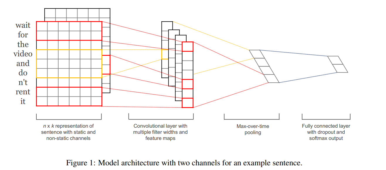
Figure 6.1: 利用词向量转写为一个 numerical representation。文本转写为一个一维图片格式，channel为词向量维度。通过 filter 后，feature map 也还是一维的，所以可以理解输入是一维图片格式。‘Convolutional layer with multiple filter widths and feature maps’ 因为 filter 可以 kernel size不一样，所以产生的 feature map 也不一样，反正最后都要 max out。

The model architecture, shown in figure \(1,\) is a slight variant of the CNN architecture of Collobert et al. \((2011) .\) Let \(\mathbf{x}_{i} \in \mathbb{R}^{k}\) be the \(k\) -dimensional word vector corresponding to the \(i\) -th word in the sentence. A sentence of length \(n\) (padded where necessary) is represented as \[ \mathbf{x}_{1: n}=\mathbf{x}_{1} \oplus \mathbf{x}_{2} \oplus \ldots \oplus \mathbf{x}_{n} \]

where \(\oplus\) is the concatenation operator. In general, let \(\mathbf{x}_{i: i+j}\) refer to the concatenation of words \(\mathbf{x}_{i}, \mathbf{x}_{i+1}, \ldots, \mathbf{x}_{i+j}\).

用\({1: n}\)表示一个句子。

A convolution operation in- volves a filter \(\mathbf{w} \in \mathbb{R}^{h k},\) which is applied to a window of \(h\) words to produce a new feature.

\(\mathbf{w} \in \mathbb{R}^{h k}\) 说明每一个通道上都有一个 filter。 h 相当于 kernel size。

For example, a feature \(c_{i}\) is generated from a window of words \(\mathbf{x}_{i: i+h-1}\) by \[ c_{i}=f\left(\mathbf{w} \cdot \mathbf{x}_{i: i+h-1}+b\right) \] Here \(b \in \mathbb{R}\) is a bias term and \(f\) is a non-linear function such as the hyperbolic tangent. This filter is applied to each possible window of words in the sentence \(\left\{\mathbf{x}_{1: h}, \mathbf{x}_{2: h+1}, \ldots, \mathbf{x}_{n-h+1: n}\right\}\) to produce a feature map \[ \mathbf{c}=\left[c_{1}, c_{2}, \ldots, c_{n-h+1}\right] \] with \(\mathbf{c} \in \mathbb{R}^{n-h+1}\).

因为 h 对每个通道可以不同，所以 feature map 大小可以不一样。

We then apply a max-overtime pooling operation (Collobert et al., 2011 ) over the feature map and take the maximum value \(\hat{c}=\max \{\mathbf{c}\}\) as the feature corresponding to this particular filter.

‘max-overtime pooling operation’ 就是直接求最大值。

The idea is to capture the most important feature-one with the highest value-for each feature map. This pooling scheme naturally deals with variable sentence lengths.

‘max-overtime pooling operation’ 就是用来处理 feature map 大小不一样的。

经过一层 filter，产生一个 feature map (类似于一张图)，多层 filter，产生多个 feature maps。 每个通道(词向量维度)对应一个filter。

然后 filter 是 max pooling 处理的，(Kim 2014) 认为局部最大值反映了最重要的特征。

We have described the process by which one feature is extracted from one filter. The model uses multiple filters (with varying window sizes)

作者的做法里面 filter 的 kernel size 是不同的。

to obtain multiple features. These features form the penultimate layer and are passed to a fully connected softmax layer whose output is the probability distribution over labels.

这个就是倒数第二层的结构了， 在 maxout 后，后面就是一个全连接的 softmax 层，直接进行多分类任务了。

In one of the model variants, we experiment with having two ‘channels’ of word vectors—one that is kept static throughout training and one that is fine-tuned via backpropagation (section 3.2).2 In the multichannel architecture, illustrated in figure 1, each filter is applied to both channels and the results are added to calculate ci in equation (2). The model is otherwise equivalent to the single channel architecture.

从图片角度理解，(Kim 2014) 用’词向量’构造了一个维度图片，(Kim 2014) 让图像有两个通道，

1. 词向量不训练的
2. 词向量训练的

这是一个小的 trick。

6.3 Results and Discussion

Results of our models against other methods are listed in table 2. Our baseline model with all randomly initialized words (CNN-rand) does not perform well on its own. While we had expected performance gains through the use of pre-trained vectors, we were surprised at the magnitude of the gains. Even a simple model with static vectors (CNN-static) performs remarkably well, giving competitive results against the more sophisticated deep learning models that utilize complex pooling schemes (Kalchbrenner et al., 2014) or require parse trees to be computed beforehand (Socher et al., 2013). These results suggest that the pretrained vectors are good, ‘universal’ feature extractors and can be utilized across datasets. Finetuning the pre-trained vectors for each task gives still further improvements (CNN-non-static)

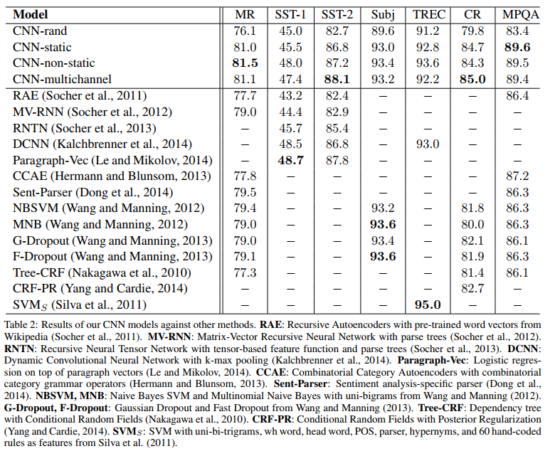
Figure 6.2: 显然随机给词向量的情况是不好的结果，加入词向量后无论是否可训练，结果都表现不错。

6.4 scratch

reticulate::use_python(Sys.which("python"))

其实，我们也可以将文本当作一维图像，从而可以用一维卷积神经网络来捕捉临近词之间的关联。本节将介绍将卷积神经网络应用到文本分析的开创性工作之一：textCNN [1]。

首先导入实验所需的包和模块。

import d2lzh as d2l
from mxnet import gluon, init, nd
from mxnet.contrib import text
from mxnet.gluon import data as gdata, loss as gloss, nn

6.4.1 一维卷积层

在介绍模型前我们先来解释一维卷积层的工作原理。与二维卷积层一样，一维卷积层使用一维的互相关运算。在一维互相关运算中，卷积窗口从输入数组的最左方开始，按从左往右的顺序，依次在输入数组上滑动。当卷积窗口滑动到某一位置时，窗口中的输入子数组与核数组按元素相乘并求和，得到输出数组中相应位置的元素。如图10.4所示，输入是一个宽为7的一维数组，核数组的宽为2。可以看到输出的宽度为\(7-2+1=6\)，且第一个元素是由输入的最左边的宽为2的子数组与核数组按元素相乘后再相加得到的：\(0\times1+1\times2=2\)。

一维互相关运算

下面我们将一维互相关运算实现在corr1d函数里。它接受输入数组X和核数组K，并输出数组Y。

def corr1d(X, K):
    w = K.shape[0]
    Y = nd.zeros((X.shape[0] - w + 1))
    for i in range(Y.shape[0]):
        Y[i] = (X[i: i + w] * K).sum()
    return Y

X, K = nd.array([0, 1, 2, 3, 4, 5, 6]), nd.array([1, 2])
X

## 
## [0. 1. 2. 3. 4. 5. 6.]
## <NDArray 7 @cpu(0)>

K

## 
## [1. 2.]
## <NDArray 2 @cpu(0)>

corr1d(X, K)

## 
## [ 2.  5.  8. 11. 14. 17.]
## <NDArray 6 @cpu(0)>

多输入通道的一维互相关运算也与多输入通道的二维互相关运算类似：在每个通道上，将核与相应的输入做一维互相关运算，并将通道之间的结果相加得到输出结果。图10.5展示了含3个输入通道的一维互相关运算，其中阴影部分为第一个输出元素及其计算所使用的输入和核数组元素：\(0\times1+1\times2+1\times3+2\times4+2\times(-1)+3\times(-3)=2\)。

含3个输入通道的一维互相关运算

def corr1d_multi_in(X, K):
    # 首先沿着X和K的第0维（通道维）遍历。然后使用*将结果列表变成add_n函数的位置参数
    #（positional argument）来进行相加
    return nd.add_n(*[corr1d(x, k) for x, k in zip(X, K)])

X = nd.array([[0, 1, 2, 3, 4, 5, 6],
              [1, 2, 3, 4, 5, 6, 7],
              [2, 3, 4, 5, 6, 7, 8]])
K = nd.array([[1, 2], [3, 4], [-1, -3]])
corr1d_multi_in(X, K)

## 
## [ 2.  8. 14. 20. 26. 32.]
## <NDArray 6 @cpu(0)>

由二维互相关运算的定义可知，多输入通道的一维互相关运算可以看作单输入通道的二维互相关运算。

这是我们大多数理解的 textCNN。

如图10.6所示，我们也可以将图10.5中多输入通道的一维互相关运算以等价的单输入通道的二维互相关运算呈现。这里核的高等于输入的高。图10.6中的阴影部分为第一个输出元素及其计算所使用的输入和核数组元素：\(2\times(-1)+3\times(-3)+1\times3+2\times4+0\times1+1\times2=2\)。

单输入通道的二维互相关运算

6.4.2 时序最大池化层

类似地，我们有一维池化层。textCNN中使用的时序最大池化（max-over-time pooling）层实际上对应一维全局最大池化层：

注意这里是全局的。

假设输入包含多个通道，各通道由不同时间步上的数值组成，各通道的输出即该通道所有时间步中最大的数值。因此， 时序最大池化层的输入在各个通道上的时间步数可以不同。

是所有时间步中最大的。

为提升计算性能，我们常常将不同长度的时序样本组成一个小批量，并通过在较短序列后附加特殊字符（如0）令批量中各时序样本长度相同。这些人为添加的特殊字符当然是无意义的。由于时序最大池化的主要目的是抓取时序中最重要的特征，它通常能使模型不受人为添加字符的影响。

因为是 maxpool 所以 padding 才可以是 0，否则 minpool 就有问题。

6.4.3 读取和预处理IMDb数据集

batch_size = 64
# d2l.download_imdb()
train_data, test_data = d2l.read_imdb('train'), d2l.read_imdb('test')
vocab = d2l.get_vocab_imdb(train_data)
train_iter = gdata.DataLoader(gdata.ArrayDataset(
    *d2l.preprocess_imdb(train_data, vocab)), batch_size, shuffle=True)
test_iter = gdata.DataLoader(gdata.ArrayDataset(
    *d2l.preprocess_imdb(test_data, vocab)), batch_size)

6.4.4 textCNN模型

textCNN模型主要使用了一维卷积层和时序最大池化层。假设输入的文本序列由\(n\)个词组成，每个词用\(d\)维的词向量表示。那么输入样本的宽为\(n\)，高为1，输入通道数为\(d\)。textCNN的计算主要分为以下几步。

1. 定义多个一维卷积核，并使用这些卷积核对输入分别做卷积计算。宽度不同的卷积核可能会捕捉到不同个数的相邻词的相关性。

宽度不同的 kernel 具备不同的 local 信息。

2. 对输出的所有通道分别做时序最大池化，再将这些通道的池化输出值连结为向量。
3. 通过全连接层将连结后的向量变换为有关各类别的输出。这一步可以使用丢弃层应对过拟合。

图10.7用一个例子解释了textCNN的设计。这里的输入是一个有11个词的句子，每个词用6维词向量表示。因此输入序列的宽为11，输入通道数为6。

词向量相当于通道，不是长度。

这里样本为 batch，词向量为通道，词语长度为宽，这里没有长，因为时序是一维的。

给定2个一维卷积核，核宽分别为2和4，输出通道数分别设为4和5。因此，一维卷积计算后，4个输出通道的宽为\(11-2+1=10\)，而其他5个通道的宽为\(11-4+1=8\)。尽管每个通道的宽不同，我们依然可以对各个通道做时序最大池化，并将9个通道的池化输出连结成一个9维向量。

因为这里的时序最大池化直接求一个通道里面序列的最大值了。 因此九个通道为九个值。

最终，使用全连接将9维向量变换为2维输出，即正面情感和负面情感的预测。

textCNN的设计

下面我们来实现textCNN模型。与上一节相比，除了用一维卷积层替换循环神经网络外，这里我们还使用了两个嵌入层，一个的权重固定，另一个的权重则参与训练。

class TextCNN(nn.Block):
    def __init__(self, vocab, embed_size, kernel_sizes, num_channels,
                 **kwargs):
        super(TextCNN, self).__init__(**kwargs)
        self.embedding = nn.Embedding(len(vocab), embed_size)
        # 不参与训练的嵌入层
        self.constant_embedding = nn.Embedding(len(vocab), embed_size)
        self.dropout = nn.Dropout(0.5)
        self.decoder = nn.Dense(2)
        # 时序最大池化层没有权重，所以可以共用一个实例
        self.pool = nn.GlobalMaxPool1D()
        self.convs = nn.Sequential()  # 创建多个一维卷积层
        for c, k in zip(num_channels, kernel_sizes):
            self.convs.add(nn.Conv1D(c, k, activation='relu'))

    def forward(self, inputs):
        # 将两个形状是(批量大小, 词数, 词向量维度)的嵌入层的输出按词向量连结
        embeddings = nd.concat(
            self.embedding(inputs), self.constant_embedding(inputs), dim=2)
        # 根据Conv1D要求的输入格式，将词向量维，即一维卷积层的通道维，变换到前一维
        embeddings = embeddings.transpose((0, 2, 1))
        # 对于每个一维卷积层，在时序最大池化后会得到一个形状为(批量大小, 通道大小, 1)的
        # NDArray。使用flatten函数去掉最后一维，然后在通道维上连结
        encoding = nd.concat(*[nd.flatten(
            self.pool(conv(embeddings))) for conv in self.convs], dim=1)
        # 应用丢弃法后使用全连接层得到输出
        outputs = self.decoder(self.dropout(encoding))
        return outputs

创建一个TextCNN实例。它有3个卷积层，它们的核宽分别为3、4和5，输出通道数均为100。

embed_size, kernel_sizes, nums_channels = 100, [3, 4, 5], [100, 100, 100]
# ctx = d2l.try_all_gpus()
net = TextCNN(vocab, embed_size, kernel_sizes, nums_channels)

# net.initialize(init.Xavier(), ctx=ctx)
net.initialize(init.Xavier())

• 没有执行起来还是要安装d2l

6.4.4.1 加载预训练的词向量

同上一节一样，加载预训练的100维GloVe词向量，并分别初始化嵌入层embedding和constant_embedding，前者权重参与训练，而后者权重固定。

glove_embedding = text.embedding.create(
    'glove', pretrained_file_name='glove.6B.100d.txt', vocabulary=vocab)
net.embedding.weight.set_data(glove_embedding.idx_to_vec)
net.constant_embedding.weight.set_data(glove_embedding.idx_to_vec)
net.constant_embedding.collect_params().setattr('grad_req', 'null')

6.5 像图像来理解文字

For example, below we define an Embedding layer with a vocabulary of 200 (e.g. integer encoded words from 0 to 199, inclusive), a vector space of 32 dimensions in which words will be embedded, and input documents that have 50 words each. The output of the Embedding layer is a 2D vector with one embedding for each word in the input sequence of words (input document).

如果batch size 有10个样本，每个样本长度 padding 后为50个词，词库有200个one-hot 后产生特征向量。 那么数据维度为(50,(10,200))(Zhang et al. 2019)。

按照(Brownlee 2017)的做法，数据维度为(10,50,200)。

经过词向量处理后变为

\[(10,50,200) \times (50,200,32) = (10,50,32) = \text{10 images}\]

textCNN 的方式就是把词向量 x 句子长度，就是一个单通道的图片了。试图理解 w2v 怎么放入 RNN 的。 其中词向量定义为e = Embedding(200, 32, input_length=50)。

(10,50,200)对应的是(batch, length, voca)，这里完成了 200 到 32 的降维，也是一种理解的方式，但是并非 TextCNN 的真正做法。

If you wish to connect a Dense layer directly to an Embedding layer, you must first flatten the 2D output matrix to a 1D vector using the Flatten layer.

flatten 的做法为

\[(10,50,32) = (10,50 \times 32)\]

参考 https://datascience.stackexchange.com/a/56449/60879

Doing this is referred to as building an embedding layer “in front of” your LSTM/RNN/GRU network model. For the embedding layer you need to specify:

1. maximum length of a sequence
2. embedding size for each token.

如果不用 Flatten 的话，也可以使用 RNN。

What will be the dimensions of Xt to feed into the LSTM? And how is the LSTM trained? If each Xt is a 100-dimension vector represent one word in a review, do I feed each word in a review to a LSTM at a time? What will LSTM do in each epoch?

这里的 RNN 的输入变成了 (词语,batch,词向量)。

参考 https://stackoverflow.com/a/50419240/8625228

Shapes with the embedding:

• Shape of the input data: X_train.shape == (reviews, words), which is (reviews, 500)

In the LSTM (after the embedding, or if you didn’t have an embedding)

• Shape of the input data: (reviews, words, embedding_size):

  • (reviews, 500, 100) - where 100 was automatically created by the embedding
    

• Input shape for the model (if you didn’t have an embedding layer) could be either:

  • input_shape = (500, 100)
    
  • input_shape = (None, 100) - This option supports variable length reviews
    

• Each Xt is a slice from input_data[:,timestep,:], which results in shape:

  • (reviews, 100)
    
  • But this is entirely automatic, made by the layer itself.
    

• Each Ht is discarded, the result is only the last h, because you’re not using return_sequences=True (but this is ok for your model).

Your code seems to be doing everything, so you don’t have to do anything special to train this model. Use fit with a proper X_train and you will get y_train with shape (reviews,1).

7 GAN

The purpose of two Networks may be summarised as to learn the underlying structure of the input database as much as possible and using that knowledge to create similar content which fits all the parameters to fit in the same category. (Raina 2019)

读懂什么是GAN，判别器，就是判断真实样本和生成样本是否一致。

As users, we know if it was from the real or fake sample, and using this knowledge we can backpropagate a training loss in order for the discriminator to do its job much better. (Raina 2019)

generator 和 discriminator 都可以一起训练。

But as we know, the Generator is a Neural-Network as well, so we can backpropagate all the way to the random sample noise and thus help generate better images. By doing this, the same loss function works for both, the discriminator and the generator as well. (Raina 2019)

因此 generator 训练后就可以产生逼真的 image 了。

The Generator and the Discriminator are in a mini-max game. (Raina 2019) Generator is trying to minimize the gap between the real and fake images so as to fool the discriminator. (Raina 2019) Discriminator is trying to maximize the understanding of real images so as to distinguish the fake samples. (Raina 2019)

Generator 是为了逼真，Discriminator 是为了加以区别。

\[\min _{G} \max _{D} \mathbb{E}_{x \sim q_{\text {data }}(x)}[\log D(\boldsymbol{x})]+\mathbb{E}_{\boldsymbol{z} \sim p(\boldsymbol{z})}[\log (1-D(G(\boldsymbol{z})))]\]

1. Minimize this loss wrt the Generator parameters
2. Maximize this loss wrt the Discriminator parameters

因此一个好的GAN，要在这两边平衡。

孙裕道 (2020)

GAN 的目标是解决以下问题：假设有一组对象数据集，例如，一组猫的图像，或者手写的汉字，或者梵高的绘画等等，GAN 可以通过噪声生成相似的对象，原理是神经网络通过使用训练数据集对网络参数进行适当调整，

这是原理。

并且深度神经网络可以用来近似任何函数。

理论上是的。

对于 GAN 判别器函数 D 和生成函数 G 建模为神经网络，其中具体 GAN 的模型如下图所示，GAN 网络实际上包含了 2 个网络，一个是生成网络 G 用于生成假样本,另一个是判别网络 D 用于判别样本的真假，并且为了引入对抗损失，通过对抗训练的方式让生成器能够生成高质量的图片。

这么看理解了，生成器可以孤立出来做预测。

Wang (2020)

7.1 Introduction

7.1.1 Background

The original GAN, which we shall refer to as the vanilla \(G A N\) in this paper, was introduced in [4] as a new generative framework from training data sets. Its goal was to address the following question: Suppose we are given a data set of objects with certain degree of consistency, for example, a collection of images of cats, or handwrit- ten Chinese characters, or Van Gogh painting etc., can we artificially generate similar objects?

产生相似的对象，这是 GAN 主要去做的事情。

This question is quite vague so we need to make it more mathematically specific. We need to clarify what do we mean by “objects with certain degree of consistency” or “similar objects”, before we can move on.

部分相似，其他风格迁移。

First we shall assume that our objects are points in \(\mathbb{R}^{n} .\) For example, a grayscale digital image of 1 megapixel can be viewed as a point in \(\mathbb{R}^{n}\) with \(n=10^{6} .\) Our data set (training data set) is simply a collection of points in \(\mathbb{R}^{n},\) which we denote by \(\mathcal{X} \subset \mathbb{R}^{n}\). When we say that the objects in the data set \(\mathcal{X}\) have certain degree of consistency we mean that they are samples generated from a common probability distribution \(\mu\) on \(\mathbb{R}^{n},\) which is often assumed to have a density function \(p(x)\). Of course by assuming \(\mu\) to have a density function mathematically we are assuming that \(\mu\) is absolutely continuous. Some mathematicians may question the wisdom of this assumption by pointing out that it is possible (in fact even likely) that the objects of interest lie on a lower dimensional manifold, making \(\mu\) a singular probability distribution. For example, consider the MNIST data set of handwritten digits. While they are \(28 \times 28\) images (so \(n=784\) ), the actual dimension of these data points may lie on a manifold with much smaller dimension (say the actual dimension may only be 20 or so). This is a valid criticism. Indeed when the actual dimension of the distribution is far smaller than the ambient dimension various problems can arise, such as failure to converge or the so-called mode collapsing, leading to poor results in some cases. Still, in most applications this assumption does seem to work well. Furthermore, we shall show that the requirement of absolute continuity is not critical to the GAN framework and can in fact be relaxed.

相似性来源于一个分布\(\mu\)，这个分布是多元的。 另外，这里假设为连续的，但是作者说事实上可以放宽一点这个假设。

另外，多维度其实可能没有必要，往往远小于我们估计的，但是太少的维度容易出现 mode collapsing，导致不好的结果。

Quantifying “similar objects” is a bit trickier and holds the key to GANs. There are many ways in mathematics to measure similarity. For example, we may define a distance function and call two pints x, y “similar” if the distance between them is small. But this idea is not useful here.

度量相似性是 GAN 的主要工作，更常见的，我们是基于距离函数完成这一步。

Our objective is not to generate objects that have small distances to some existing objects in \(\mathcal{X}\). Rather we want to generate new objects that may not be so close in whatever distance measure we use to any existing objects in the training data set \(\mathcal{X},\) but we feel they belong to the same class.

但是 GAN 的做法不是去找训练集里面最近的样本，而是和训练集的样本不那么’近’，但是看起来是一类的。

A good analogy is we have a data set of Van Gogh paintings. We do not care to generate a painting that is a perturbation of Van Gogh’s Starry Night. Instead we would like to generate a painting that a Van Gogh expert will see as a new Van Gogh painting she has never seen before.

就是一个生成的作用。

A better angle, at least from the perspective of GANs, is to define similarity in the sense of probability distribution. Two data sets are considered similar if they are samples from the same (or approximately same) probability distribution. Thus more specifically we have our training data set \(\mathcal{X} \subset \mathbb{R}^{n}\) consisting of samples from a probability distribution \(\mu\) (with density \(p(\mathbf{x})\) ), and we would like to find a probability distribution \(\nu\) (with density \(q(\mathbf{x})\) ) such that \(\nu\) is a good approximation of \(\mu .\) By taking samples from the distribution \(\nu\) we obtain generated objects that are “similar” to the objects in \(\mathcal{X}\).

GAN 的实现方式是把相似性用分布进行度量。 假设有分布 \(\mu\) 和 \(\nu\)，只要 \(\nu\) 是很好的相似分布，那么从 \(\nu\) 出来的样本就是很好的样本了。

7.1.2 The Basic Approach of GAN

The approach taken by the vanilla GAN is to form an adversarial system from which \(G\) continues to receive updates to improve its performance. More precisely it introduces a “discriminator function” \(D(x),\) which tries to dismiss the samples generated by \(G\) as fakes. The discriminator \(D(x)\) is simply a classifier that tries to distinguish samples in the training set \(\mathcal{X}\) (real samples) from the generated samples \(G(\mathbf{z})\) (fake samples). It assigns to each sample \(\mathbf{x}\) a probability \(D(\mathbf{x}) \in[0,1]\) for its likelihood to be from the same distribution as the training samples. When samples \(G\left(\mathbf{z}_{j}\right)\) are generated by \(G,\) the discriminator \(D\) tries to reject them as fakes. In the beginning this shouldn’t be hard because the generator \(G\) is not very good. But each time \(G\) fails to generate samples to fool \(D,\) it will learn and adjust with an improve- ment update. The improved \(G\) will perform better, and now it is the discriminator \(D\) ’s turn to update itself for improvement. Through this adversarial iterative process an equilibrium is eventually reached, so that even with the best discriminator \(D\) it can do no better than random guess. At such point, the generated samples should be very similar in distribution to the training samples \(\mathcal{X}\).

整个实现过程中 \(G(\mathbf{z})\) 生成假样本，\(D\) 进行判断，一开始简单，所以很容易判断，那么 \(G(\mathbf{z})\) 进行调整，直到 \(D\) 不能区分。然后 \(D\) 又加强训练。这样周而复始，知道 \(D\) 不能比随机更好，那么这时 \(G(\mathbf{z})\) 生成的样本就可以以假乱真了。

So one may ask: where do neural networks and deep learning have to do with all this? The answer is that we basically have the fundamental faith that deep neural networks can be used to approximate just about any function, through proper tuning of the network parameters using the training data sets. In particular neural networks excel in classification problems. Not surprisingly, for GAN we shall model both the discriminator function \(D\) and the generator function \(G\) as neural networks with parameters \(\omega\) and \(\theta\), respectively. Thus we shall more precisely write \(D(x)\) as \(D_{\omega}(x)\) and \(G(z)\) as \(G_{\theta}(z),\) and denote \(\nu_{\theta}:=\gamma \circ G_{\theta}^{-1}\). Our objective is to find the desired \(G_{\theta}(\mathbf{z})\) by properly tuning \(\theta\)

为了让 \(\nu\) 和 \(\mu\) 类似，因此我们需要一个算法能够拟合任何分布出来，正好就是神经网络。

7.2 Mathematical Formulation of the Vanilla GAN

The adversarial game described in the previous section can be formulated mathe- matically by minimax of a target function between the discriminator function \(D(x):\) \(\mathbb{R}^{n} \longrightarrow[0,1]\) and the generator function \(G: \mathbb{R}^{d} \longrightarrow \mathbb{R}^{n} .\) The generator \(G\) turns random samples \(\mathbf{z} \in \mathbb{R}^{d}\) from distribution \(\gamma\) into generated samples \(G(\mathbf{z})\). The discriminator \(D\) tries to tell them apart from the training samples coming from the distribution \(\mu\) while \(G\) tries to make the generated samples as similar in distribution to the training samples. In [4] a target loss function is proposed to be \[ V(D, G):=\mathbb{E}_{\mathbf{x} \sim \mu}[\log D(\mathbf{x})]+\mathbb{E}_{\mathbf{z} \sim \gamma}[\log (1-D(G(\mathbf{z})))] \] where \(\mathbb{E}\) denotes the expectation with respect to a distribution specified in the sub- script. When there is no confusion we may drop the subscript. The vanilla GAN solves the minimax problem \[\min _{G} \max _{D} V(D, G):=\min _{G} \max _{D}\left(\mathbb{E}_{\mathbf{x} \sim \mu}[\log D(\mathbf{x})]+\mathbb{E}_{\mathbf{z} \sim \gamma}[\log (1-D(G(\mathbf{z})))]\right)\]

如何理解 mini-max。按照章节7.1.2，\(D\)为了最大似然估计(因此 max)，然后\(G\)为了最像训练集(因此 mini)

Intuitively, for a given generator \(G, \max _{D} V(D, G)\) optimizes the discriminator \(D\) t reject generated samples \(G(\mathbf{z})\) by attempting to assign high values to samples from the distribution \(\mu\) and low values to generated samples \(G(\mathbf{z})\).

更加具体地， 让\(\hat y \to 1\) 的情况更符合分布 \(\mu\) 让\(\hat y \to 0\) 的情况更符合分布 \(\nu\) 或者 \(G(\mathbf{z})\) 产生的样本

Conversely, for a giver discriminator \(D, \min _{G} V(D, G)\) optimizes \(G\) so that the generated samples \(G(\mathbf{z})\) wil attempt to “fool” the discriminator \(D\) into assigning high values.

Now set \(\mathbf{y}=G(\mathbf{z}) \in \mathbb{R}^{n},\) which has distribution \(\nu:=\gamma \circ G^{-1}\) as \(\mathbf{z} \in \mathbb{R}^{d}\) has distribution \(\gamma\). We can now rewrite \(V(D, G)\) in terms of \(D\) and \(\nu\) as \[ \begin{aligned} \tilde{V}(D, \nu):=V(D, G) &=\mathbb{E}_{\mathbf{x} \sim \mu}[\log D(\mathbf{x})]+\mathbb{E}_{\mathbf{z} \sim \gamma}[\log (1-D(G(\mathbf{z})))] \\ &=\mathbb{E}_{\mathbf{x} \sim \mu}[\log D(\mathbf{x})]+\mathbb{E}_{\mathbf{y} \sim \nu}[\log (1-D(\mathbf{y}))] \end{aligned} \] (2.3) \[ =\int_{\mathbb{R}^{n}} \log D(x) d \mu(x)+\int_{\mathbb{R}^{n}} \log (1-D(y)) d \nu(y) \]

7.3 Alternative to GAN: Variational Autoencoder (VAE)

作者把 GAN 和 VAE 讨论起来。

Variational Autoencoder (VAE) is an alternative generative model to GAN. To understand VAE one needs to first understand what is an autoencoder. In a nutshell an autoencoder consists of an encoder neural network \(F\) that maps a dataset \(\mathcal{X} \subset \mathbb{R}^{n}\) to \(\mathbb{R}^{d},\) where \(d\) is typically much smaller than \(n,\) together with a decoder neural network \(H\) that “decodes” elements of \(\mathbb{R}^{d}\) back to \(\mathbb{R}^{n}\). In other words, it encodes the \(n\) -dimensional features of the dataset to the \(d\) -dimensional latents, along with a way to convert the latents back to the features. Autoencoders can be viewed as data compressors that compress a higher dimensional dataset to a much lower dimensional data set without losing too much information. For example, the MNIST dataset consists of images of size \(28 \times 28,\) which is in \(\mathbb{R}^{784}\). An autoencoder can easily compress it to a data set in \(\mathbb{R}^{10}\) using only 10 latents without losing much information. A typical autoencoder has a “bottleneck” architecture, which is shown in Figure \(1 .\) The loss function for training an autoencoder is typically the mean square error \((\mathrm{MSE})\) \[ \mathbf{L}_{\mathrm{AE}}:=\frac{1}{N} \sum_{\mathbf{x} \in \mathcal{X}}\|H(F(\mathbf{x}))-\mathbf{x}\|^{2} \]

GAN 和 AE 都是无监督学习。

其他 GAN 的变形，放到之后遇到具体模型后再学习。

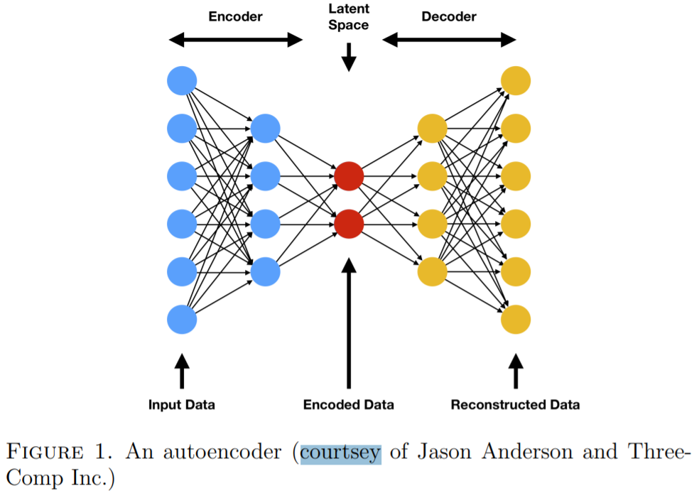
Figure 7.1: 了解 VAE 先要了解 AE，AE 具备了瓶颈。

where \(N\) is the size of \(\mathcal{X}\). For binary data we may use the Bernoulli Cross Entropy \((\mathrm{BCE})\) loss function. Furthermore, we may also add a regularization term to force desirable properties, e.g. a LASSO style \(L^{1}\) loss to gain sparsity.

First developed in \([7],\) VAEs are also neural networks having similar architectures as autoencoders, with stochasticity added into the networks. Autoencoders are deterministic networks in the sense that output is completely determined by the input. To make generative models out of autoencoders we will need to add ran- domness to latents. In an autoencoder, input data \(\mathrm{x}\) are encoded to the latents \(\mathbf{z}=F(\mathbf{x}) \in \mathbb{R}^{d},\) which are then decoded to \(\hat{\mathbf{x}}=H(F(\mathbf{z})) .\) A VAE deviates from an autoencoder in the following sense: the input \(\mathbf{x}\) is encoded into a diagonal Gaussian random variable \(\boldsymbol{\xi}=\boldsymbol{\xi}(\mathbf{x})\) in \(\mathbb{R}^{d}\) with mean \(\boldsymbol{\mu}(\mathbf{x})\) and variance \(\boldsymbol{\sigma}^{2}(\mathbf{x})\). Here \(\boldsymbol{\sigma}^{2}(\mathbf{x})=\left[\sigma_{1}^{2}(\mathbf{x}), \ldots, \sigma_{d}^{2}(\mathbf{x})\right]^{T} \in \mathbb{R}^{d}\) and the variance is actually \(\operatorname{diag}\left(\boldsymbol{\sigma}^{2}\right) .\) Another way to look at this setup is that instead of having just one encoder \(F\) in an autoencoder, a VAE neural network has two encoders \(\boldsymbol{\mu}\) and \(\boldsymbol{\sigma}^{2}\) for both the mean and the vari- ance of the latent variable \(\boldsymbol{\xi}\). As in an autoencoder, it also has a decoder \(H\). With randomness in place we now have a generative model.

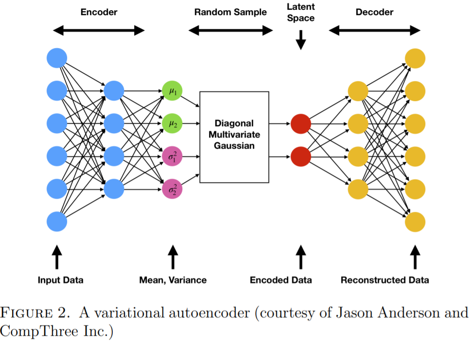
Figure 7.2: VAE 相比较于 AE，多了随机性，并且有两个 encoders \(\boldsymbol{\mu}\) 和 \(\boldsymbol{\sigma}^{2}\)。

8 PR 和 ROC 的关系

Receiver Operator Characteristic (ROC) curves are commonly used to present results for binary decision problems in machine learning. However, when dealing with highly skewed datasets, Precision-Recall (PR) curves give a more informative picture of an algorithm’s performance.

• 这里的 skew 如何定义？

skew

This difference exists because in this domain the number of negative examples greatly exceeds the number of positives examples.

这里的 ‘skew’ 指的是不平衡样本，这里指的是 ‘more informative’，但是并非是 better。因为 PR 最优化的情况下，ROC 也可以是异常的。

Furthermore, algorithms that optimize the area under the ROC curve are not guaranteed to optimize the area under the PR curve.

ROC-AUC最大化和PR-AUC最大化不是一致的，但是是单调的。

(Davis and Goadrich 2006)的证明涉及到很多统计知识 convex set，这里忽略。

8.1 Introduction

They recommended when evaluating binary decision problems to use Receiver Operator Characteristic (ROC) curves, which show how the number of correctly classified positive examples varies with the number of incorrectly classified negative examples. However, ROC curves can present an overly optimistic view of an algorithm’s performance if there is a large skew in the class distribution.

• 所以回到 AUC 的研究，当样本不平衡的时候，AUC 和 KS 都有效(work)，但是不是完全的(totally work)。

因为(Cortes and Mohri 2004)也论证了当样本不平衡严重时，重复抽样下AUC的方差变大，因此一个特定的树、特定的模型，AUC会落到比较差的情况去。

Sample ROC curves and PR curves are shown in Figures 1(a) and 1(b) respectively. These curves, taken from the same learned models on a highly-skewed cancer detection dataset, highlight the visual difference between these spaces (Davis et al., n.d.). The goal in ROC space is to be in the upper-left-hand corner, and when one looks at the ROC curves in Figure 1(a) they appear to be fairly close to optimal. In PR space the goal is to be in the upper-right-hand corner, and the PR curves in Figure 1(b) show that there is still vast room for improvement.

• (Davis et al., n.d.)很有意思的图，但是没有做过多的解释。

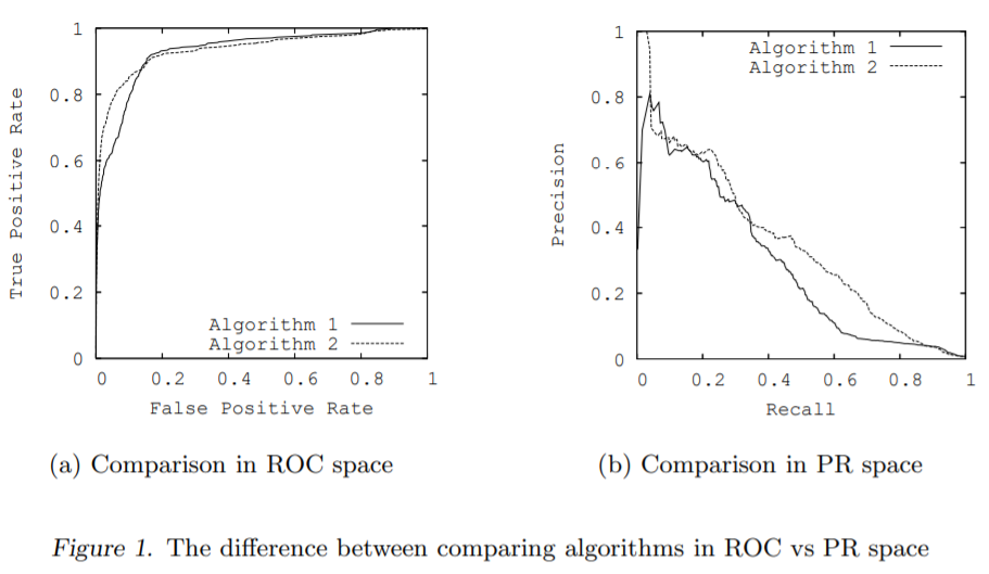
Figure 8.1: ROC 曲线表现很好，但是 PR 曲线表现很差。

Consequently, a large change in the number of false positives can lead to a small change in the false positive rate used in ROC analysis. Precision, on the other hand, by comparing false positives to true positives rather than true negatives, captures the effect of the large number of negative examples on the algorithm’s performance. Section 2 defines Precision and Recall for the reader unfamiliar with these terms.

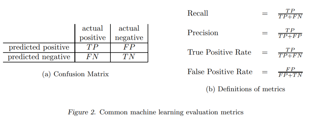
Figure 8.2: 因此问题就回到 FP 的成本上，因为负样本很多的话，很容易产生很多 FP，然而 FPR 分子和分母上区别不开，敏感度很小的话，ROC 就识别不出来。

Drummond and Holte (2000; 2004) have recommended using cost curves to address this issue. Cost curves are an excellent alternative to ROC curves, but discussing them is beyond the scope of this paper

所以要用成本矩阵来处理，来多惩罚FP(ROC的x轴)，但是这就产生一个新问题，多少的权重呢？

Based on this equivalence for ROC and PR curves, we show that a curve dominates in ROC space if and only if it dominates in PR space.

单调性不会变，但是程度意义不一样了。

8.2 Optimizing Area Under the Curve

Cortes and Mohri (2003) show that the boosting algorithm RankBoost (Freund et al., 1998) is also well-suited to optimize the AUC-ROC⁴.

(Davis and Goadrich 2006)也提及了使用排序思想(而非分类思想)来AUC优化问题。

9 AUC 在多分类上面的应用

HMC

这是 HMC 和 softmax 的差异。

Obviously, the hierarchy introduces dependencies between the classes.

We conclude that HMC trees should definitely be considered in HMC tasks where interpretable models are desired.

(Vens et al. 2008)也做了可视化方面的工作。

但是本身这个 idea 是十分好理解的，我们更多的聚焦在如何求解多分类下评价指标，这里是使用到 AUC 的变形。

9.1 Introduction

Classification refers to the task of learning from a set of classified instances a model that can predict the class of previously unseen instances. Hierarchical multi-label classification (HMC) differs from normal classification in two ways: (1) a single example may belong to multiple classes simultaneously; and (2) the classes are organized in a hierarchy: an example that belongs to some class automatically belongs to all its superclasses (we call this the hierarchy constraint).

superclasses

class 的层次结构。

Several methods can be distinguished that handle HMC tasks. A first approach transforms an HMC task into a separate binary classification task for each class in the hierarchy and applies an existing classification algorithm. We refer to it as the SC (single-label classification) approach. This technique has several disadvantages. First, it is inefficient, because the learner has to be run |C| times, with |C| the number of classes, which can be hundreds or thousands in some applications. Second, it often results in learning from strongly skewed class distributions: in typical HMC applications classes at lower levels of the hierarchy often have very small frequencies, while (because of the hierarchy constraint) the frequency of classes at higher levels tends to be very high. Many learners have problems with strongly skewed class distributions (Weiss and Provost 2003). Third, from the knowledge discovery point of view, the learned models identify features relevant for one class, rather than identifying features with high overall relevance. Finally, the hierarchy constraint is not taken into account, i.e. it is not automatically imposed that an instance belonging to a class should belong to all its superclasses.

SC

类似于对 y 变量进行了 one-hot。

A second approach is to adapt the SC method, so that this last issue is dealt with. Some authors have proposed to hierarchically combine the class-wise models in the prediction

stage, so that a classifier constructed for a class c can only predict positive if the classifier for the parent class of c has predicted positive (Barutcuoglu et al. 2006; Cesa-Bianchi et al. 2006). In addition, one can also take the hierarchy constraint into account during training by restricting the training set for the classifier for class c to those instances belonging to the parent class of c (Cesa-Bianchi et al. 2006). This approach is called the HSC (hierarchical single-label classification) approach throughout the text.

HSC

把 superclass 信息放到信息里面。然而是一个条件概率，只有当 superclass 是正的时候，才会触发 class。

A third approach is to develop learners that learn a single multi-label model that predicts all the classes of an example at once (Clare 2003; Blockeel et al. 2006). Next to taking the hierarchy constraint into account, this approach is also able to identify features that are relevant to all classes. We call this the HMC approach.

• 目前的问题是无法确定三种方法的差异

9.2 Related work

Barutcuoglu et al. (2006) recently presented a two-step approach where support vector machines (SVMs) are learned for each class separately, and then combined using a Bayesian network model so that the predictions are consistent with the hierarchy constraint.

• 就是两步法，是一个 stacking 的结构。

9.3 Predictive performance measures

9.3.1 Hierarchical loss

Cesa-Bianchi et al. (2006) have defined a hierarchical loss function that considers mistakes made at higher levels in the class hierarchy more important than mistakes made at lower levels. The hierarchical loss function for an instance \(x_{k}\) is defined as follows:

\[ \label{hierarchicalloss} l_{H}\left(x_{k}\right)=\sum_{i}\left[v_{k, i} \neq y_{k, i} \text { and } \forall c_{j} \leq_{h} c_{i}: v_{k, j}=y_{k, j}\right] \]

where \(i\) iterates over all class labels, \(v\) represents the predicted class vector, and \(y\) the real class vector. In the work of Cesa-Bianchi et al., the class hierarchy is structured as a tree, and thus, it penalizes the first mistake along the path from the root to a node. In the case of a DAG, the loss function can be generalized in two different ways. One can penalize a mistake if all ancestor nodes are predicted correctly (in this case, the above definition carries over), or one can penalize a mistake if there exists a correctly predicted path from the root to the node.

In the rest of the article, we do not consider this evaluation function, since it requires thresholded predictions, and we are interested in evaluating our methods regardless of any threshold.

公式显示损失函数中根指向节点时，判断上需要阈值。

9.3.2 Precision-recall based evaluation

Precision and recall are traditionally defined for a binary classification task with positive and negative classes. Precision is the proportion of positive predictions that are correct, and recall is the proportion of positive examples that are correctly predicted positive. That is,

\[ \text { Prec }=\frac{T P}{T P+F P}, \quad \text { and } \quad \operatorname{Rec}=\frac{T P}{T P+F N} \]

with \(T P\) the number of true positives (correctly predicted positive examples), \(F P\) the number of false positives (positive predictions that are incorrect), and \(F N\) the number of false negatives (positive examples that are incorrectly predicted negative). Note that these measures ignore the number of correctly predicted negative examples.

Although a PR curve helps in understanding the predictive behavior of the model, a single performance score is more useful to compare models. A score often used to this end is the area between the PR curve and the recall axis, the so-called “area under the PR curve” (AUPRC). The closer the AUPRC is to 1.0, the better the model is.

AUPRC

area under the PR curve。 针对 PR 曲线，对应着 AUPRC，其实和(Davis and Goadrich 2006)统一，采用AUC-ROC更容易记忆。

The reason why we believe PR curves to be a more suitable evaluation measure in this context is the following. In HMC datasets, it is often the case that individual classes have few positive instances. For example, in functional genomics, typically only a few genes have a particular function. This implies that for most classes, the number of negative instances by far exceeds the number of positive instances. We are more interested in recognizing the positive instances (that an instance has a given label), rather than correctly predicting the negative ones (that an instance does not have a particular label). Although ROC curves are better known, we believe that they are less suited for this task, exactly because they reward a learner if it correctly predicts negative instances (giving rise to a low false positive rate). This can present an overly optimistic view of the algorithm’s performance. This effect has been convincingly demonstrated and studied by (Davis and Goadrich 2006), and we refer to them for further details.

正如 PR 的定义，PR 更加关注正样本，然而 ROC 相对地，更加关注负样本，因此在这里 PR 更加适合。

• 查询 (Davis and Goadrich 2006)

A final point to note is that PR curves can be constructed for each individual class in a multi-label classification task by taking as positives the examples belonging to the class and as negatives the other examples. How to combine the class-wise performances in order to quantify the overall performance, is less straightforward. The following two paragraphs discuss two approaches, each of which are meaningful.

并且 one vs rest 的思路上，都是正样本对比所有其他样本，因此 PR 也更加合适。

• 那么如何把多个 PR 合并成一个整体指标呢？

9.3.2.1 Area under the average PR curve

A first approach to obtain an overall performance score is to construct an overall PR curve by transforming the multi-label problem into a binary problem as follows (Yang 1999 ; Tsoumakas and Vlahavas 2007; Blockeel et al. 2006). Consider a binary classifier that takes as input an (instance, class) couple and predicts whether that instance belongs to that class or not. Precision is then the proportion of positively predicted couples that are positive and recall is the proportion of positive couples that are correctly predicted positive. A rank classifier (which predicts how likely it is that the instance belongs to the class) can be turned into such a binary classifier by choosing a threshold, and by varying this threshold a PR curve is obtained. We will evaluate our predictive model in exactly the same way as such a rank classifier.

For a given threshold value, this yields one point (Prec, Rec) in PR space, which can be computed as follows: \[ \overline{\operatorname{Prec}}=\frac{\sum_{i} T P_{i}}{\sum_{i} T P_{i}+\sum_{i} F P_{i}}, \quad \text { and } \quad \overline{\operatorname{Rec}}=\frac{\sum_{i} T P_{i}}{\sum_{i} T P_{i}+\sum_{i} F N_{i}} \] where \(i\) ranges over all classes. (This corresponds to micro-averaging the precision and recall.) In terms of the original problem definition, Prec corresponds to the proportion of predicted labels that are correct and \(\overline{\operatorname{Rec}}\) to the proportion of labels in the data that are correctly predicted.

(Vens et al. 2008)使用了’micro-averaging’进行 PR。

By varying the threshold, we obtain an average PR curve. We denote the area under this curve with \(\mathrm{AU}(\overline{\mathrm{PRC}})\)

9.3.2.2 Average area under the PR curves

A second approach is to take the (weighted) average of the areas under the individual (per class) PR curves, computed as follows: \[ \overline{\mathrm{AUPRC}}_{w_{1}, \ldots, w_{|C|}}=\sum_{i} w_{i} \cdot \mathrm{AUPRC}_{i} \] The most obvious instantiation of this approach is to set all weights to \(1 /|C|,\) with \(C\) the set of classes. In the results, we denote this measure with AUPRC. A second instantiation is to weigh the contribution of a class with its frequency, that is, \(w_{i}=v_{i} / \sum_{j} v_{j},\) with \(v_{i} c_{i}\) ’s frequency in the data. The rationale behind this is that for some applications more frequent classes may be more important. We denote the latter measure with \(\overline{\mathrm{AUPRC}}_{w}\). A corresponding PR curve that has precisely \(\overline{\mathrm{AUPRC}}_{w_{1}, \ldots, w_{|C|}}\) as area can be drawn by taking, for each value on the recall axis, the (weighted) point-wise average of the class-wise precision values. Note that the interpretation of this curve is different from that of the microaveraged PR curve defined in the previous section. For example, each point on this curve may correspond to a different threshold for each class. Section 6.3 presents examples of both types of curves and provides more insight in the difference in interpretation.

第二种方法会加剧少样本的准确率。

并且这里可以利用 PoE(???) 进行强化，并且在多分类场景中PRODLDA(???)也进行了尝试。

\(\mathrm{AU}(\overline{\mathrm{PRC}}), \overline{\mathrm{AUPRC}},\) 和 \(\overline{\mathrm{AUPRC}}_{w}\)，三者差异都在 ave 上的处理。

Because of their sequential nature, RNNs are good at capturing the local structure of a word sequence – both semantic and syntactic – but might face difficulty remembering long-range dependencies.

(Dieng et al. 2016)考虑加入 RNN 的框架的目的是使用 RNN 提取 local feature 的能力。

these long-range dependencies are of semantic nature.

‘LONG-RANGE SEMANTIC DEPENDENCY’ 隐含的就是 LDA 的思想(Blei, Ng, and Jordan 2003)。

Unlike previous work on contextual RNN language modeling, our model is learned endto-end.

TopicRNN 创新上就是端到端的学习。

9.4 INTRODUCTION

These topics provide context to the RNN. Contextual RNNs have received a lot of attention (Mikolov and Zweig, 2012; Mikolov et al., 2014; Ji et al., 2015; Lin et al., 2015; Ji et al., 2016; Ghosh et al., 2016). However, the models closest to ours are the contextual RNN model proposed by Mikolov and Zweig (2012) and its most recent extension to the long-short term memory (LSTM) architecture (Ghosh et al., 2016).

• 可以了解下这些论文的 idea
• 那么以前的 contextual RNNs 有什么问题呢？

(Dieng et al. 2016)这里把contextual RNNs特指一般的语言模型，用 topicrnn 在 rnns 预测的效果去类比，而非用其主题模型的特点去和语言模型比，两者是没法比较的，功能和目的都不同。

These models use pre-trained topic model features as an additional input to the hidden states and/or the output of the RNN.

模型并非是端到端的。

We introduce an automatic way for handling stop words that topic models usually have difficulty dealing with.

停用词是主题模型很难处理的一个问题。

The remainder of the paper is organized as follows: Section 2 provides background on RNN-based language models and probabilistic topic models. Section 3 describes the TopicRNN network architecture, its generative process and how to perform inference for it. Section 4 presents per-word perplexity results on the Penn TreeBank dataset and the classification error rate on the IMDB 100K dataset. Finally, we conclude and provide future research directions in Section 5.

关注章节9.6。

9.5 BACKGROUND

9.6 THE TOPICRNN MODEL

Instead of using the Dirichlet distribution, we choose the Gaussian distribution. This allows for more flexibility in the sequence prediction problem and also has advantages during inference

作者这里使用的是高斯分布而非迪利克雷分布。

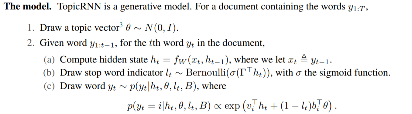
Figure 9.1: TopicRNN 结构。

The stop word indicator \(l_{t}\) controls how the topic vector \(\theta\) affects the output. If \(l_{t}=1\) (indicating \(y_{t}\) is a stop word \(),\) the topic vector \(\theta\) has no contribution to the output. Otherwise, we add a bias to favor those words that are more likely to appear when mixing with \(\theta,\) as measured by the dot product between \(\theta\) and the latent word vector \(b_{i}\) for the \(i\) th vocabulary word.

这个停用词的处理方式和HMMLDA(Griffiths et al. 2005)类似。

Unlike Mikolov and Zweig (2012), the contextual information is not passed to the hidden layer of the RNN. The main reason behind our choice of using the topic vector as bias instead of passing it into the hidden states of the RNN is because it enables us to have a clear separation of the contributions of global semantics and those of local dynamics

作者并没有把 \(\theta\) 放到隐藏层而是作为 bias，进行加权的，这样为了区分 LDA 和 RNN 各自的效果。

The global semantics come from the topics which are meaningful when stop words are excluded. However these stop words are needed for the local dynamics of the language model

依然是 HMMLDA 的 idea。

We hence achieve this separation of global vs local via a binary decision model for the stop words

我感觉就是把 HMMLDA 部分的 HMM 替换成了 RNN，并且把 \(\theta\) 作为 bias 而非隐藏层更加体现了 HMMLDA 的思想。

It is unclear how to achieve this if we pass the topics to the hidden states of the RNN. This is because the hidden states of the RNN will account for all words (including stop words) whereas the topics exclude stop words.

作者对 \(\theta\) 放到 bias 还是很有学术创新的。

Figure 9.2: (Dieng et al. 2016)对待停用词的思想和(Griffiths et al. 2005)对待function words的思想差不多。

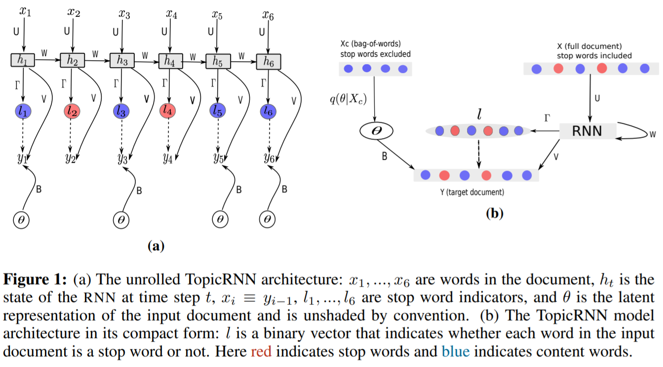
We show the unrolled graphical representation of TopicRNN in Figure 1 (a). We denote all model parameters as \(\Theta=\left\{\Gamma, V, B, W, W_{c}\right\}\) (see Appendix A. 1 for more details). Parameter \(W_{c}\) is for the inference network, which we will introduce below. The observations are the word sequences \(y_{1: T}\) and stop word indicators \(l_{1: T} \cdot{ }^{4}\) The log marginal likelihood of the sequence \(y_{1: T}\) is \[ \log p\left(y_{1: T}, l_{1: T} \mid h_{t}\right)=\log \int p(\theta) \prod_{t=1}^{T} p\left(y_{t} \mid h_{t}, l_{t}, \theta\right) p\left(l_{t} \mid h_{t}\right) \mathrm{d} \theta \]

content word seq 和 stop word seq 都是输出层。

9.7 EXPERIMENTS

Our code will be made publicly available for reproducibility

• 找作者可复现的 code topicrnn

We use RNN, LSTM, and GRU cells in our experiments leading to TopicRNN, TopicLSTM, and TopicGRU.

9.8 DISCUSSION AND FUTURE WORK

In future work, we will study the performance of TopicRNN when stop words are dynamically discovered during training.

停用词作为输出层这是一个改进方向。

参考文献

Blei, David M. 2012. “Probabilistic Topic Models.” Commun. ACM 55 (4): 77–84. https://doi.org/10.1145/2133806.2133826.

Blei, David M, Andrew Y Ng, and Michael I Jordan. 2003. “Latent Dirichlet Allocation.” Journal of Machine Learning Research 3 (Jan): 993–1022.

Brownlee, Jason. 2017. “How to Use Word Embedding Layers for Deep Learning with Keras.” Machine Learning Mastery. 2017. https://machinelearningmastery.com/use-word-embedding-layers-deep-learning-keras/.

Cortes, Corinna, and Mehryar Mohri. 2004. “AUC Optimization Vs. Error Rate Minimization.” In Advances in Neural Information Processing Systems, 313–20.

Davis, Jesse, Elizabeth S Burnside, David Page, Raghu Ramakrishnan, Vitor Santos Costa, and Jude W Shavlik. n.d. “View Learning for Statistical Relational Learning: With an Application to Mammography.” In. Citeseer.

Davis, Jesse, and Mark Goadrich. 2006. “The Relationship Between Precision-Recall and Roc Curves.” In Proceedings of the 23rd International Conference on Machine Learning, 233–40.

Dieng, Adji B, Chong Wang, Jianfeng Gao, and John Paisley. 2016. “Topicrnn: A Recurrent Neural Network with Long-Range Semantic Dependency.” arXiv Preprint arXiv:1611.01702.

Griffiths, Thomas L, Mark Steyvers, David M Blei, and Joshua B Tenenbaum. 2005. “Integrating Topics and Syntax.” In Advances in Neural Information Processing Systems, 537–44.

Huang, Bo, Yan Yang, Amjad Mahmood, and Hongjun Wang. 2012. “Microblog Topic Detection Based on Lda Model and Single-Pass Clustering.” In International Conference on Rough Sets and Current Trends in Computing, 166–71. Springer.

Kim, Yoon. 2014. “Convolutional Neural Networks for Sentence Classification.” In Proceedings of the 2014 Conference on Empirical Methods in Natural Language Processing (EMNLP), 1746–51. Doha, Qatar: Association for Computational Linguistics. https://doi.org/10.3115/v1/D14-1181.

Lin, Min, Qiang Chen, and Shuicheng Yan. 2013. “Network in Network.” arXiv Preprint arXiv:1312.4400.

Papka, Ron, James Allan, and others. 1998. “On-Line New Event Detection Using Single Pass Clustering.” University of Massachusetts, Amherst 10 (290941.290954).

Raina, Rudra. 2019. “Face-Morphing Using Generative Adversarial Network(GAN).” AI研习社. 2019. https://www.yanxishe.com/TextTranslation/2241.

Schuster, M., and K. K. Paliwal. 1997. “Bidirectional Recurrent Neural Networks.” IEEE Transactions on Signal Processing 45 (11): 2673–81.

Vens, Celine, Jan Struyf, Leander Schietgat, Sašo Džeroski, and Hendrik Blockeel. 2008. “Decision Trees for Hierarchical Multi-Label Classification.” Machine Learning 73 (2): 185.

Wang, Yang. 2020. “A Mathematical Introduction to Generative Adversarial Nets (Gan).” arXiv Preprint arXiv:2009.00169.

Zhang, Aston, Zachary C. Lipton, Mu Li, and Alexander J. Smola. 2019. Dive into Deep Learning.

孙裕道. 2020. “生成对抗网络（GAN）的数学原理全解.” PaperWeekly. 2020. https://mp.weixin.qq.com/s/iqCMA7E_vtdymVxxz7bpRA.

---

1. 作者为了区别开来ROC和PR曲线下分别的AUC。↩︎

2. 这部分参考 https://github.com/HaowenHOU/single-pass-clustering-for-chinese-text↩︎

3. 三作是大佬，主要 idea 就是在 Single Pass 里面用 LDA 替换 VSM。‘We propose a novel topic detection technique we adopt Single-pass Clustering technique by using Latent Dirichlet Allocation (LDA) Model in place of traditional VSM model, to extract the hidden microblog topics information.’↩︎

4. 作者为了区别开来ROC和PR曲线下分别的AUC。↩︎