spatialAnalysis

Moran I statistic

DataCamp

Pick any two boroughs that are neighbors - with a shared border - and the chances are they’ll be more similar than any two random boroughs.

… when using statistical models that assume, conditional on the model, that the data points are independent.

Computing these measures first requires you to work out which regions are neighbors via the poly2nb() function.

Then you can compute the test statistic and run a significance test on the null hypothesis of no spatial correlation.

input 还是需要是 sp

# Use the spdep package
library(spdep)

# Make neighbor list
borough_nb <- poly2nb(london_ref)

# Get center points of each borough
borough_centers <- coordinates(london_ref)

# Show the connections
plot(london_ref); plot(borough_nb, borough_centers, add = TRUE)

# Map the total pop'n
spplot(london_ref, zcol = "TOTAL_POP")

# Run a Moran I test on total pop'n
moran.test(
  london_ref$TOTAL_POP, 
  nb2listw(borough_nb)
)

# Map % Remain
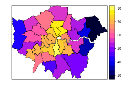
spplot(london_ref, zcol = "Pct_Remain")

# Run a Moran I MC test on % Remain
moran.mc(
  london_ref$Pct_Remain, 
  nb2listw(borough_nb), 
  nsim = 999
)

这是完整的 code， 可以使用 MC 的方式进行验证。

这里验证了两个变量是否有空间滞后性。 实际上不是所有变量都有空间滞后性的。

对于变量Pct_Remain来说，邻近区域表现出相同颜色。

可视化是理解一种特征工程最好的方式，以下图展示了为什么有空间滞后性。

knitr::include_graphics("figure/moran_i_test_plot.png")