面板数据 学习笔记
2020-04-22
面板数据英文里面可以叫做 longitudinal data,也就是经济学里面的 panel data。
1 面板数据的展示

Figure 1.1: 纵向数据的定义是个体在时间上重复进行测量后的数据。(Tierney 2020)
knitr::include_graphics("../figure/A23668EF-FB83-4574-AD1A-99AA8772B71F.jpeg")
knitr::include_graphics("../figure/807EA1D2-65EC-4000-9095-E7133757B659.jpeg")
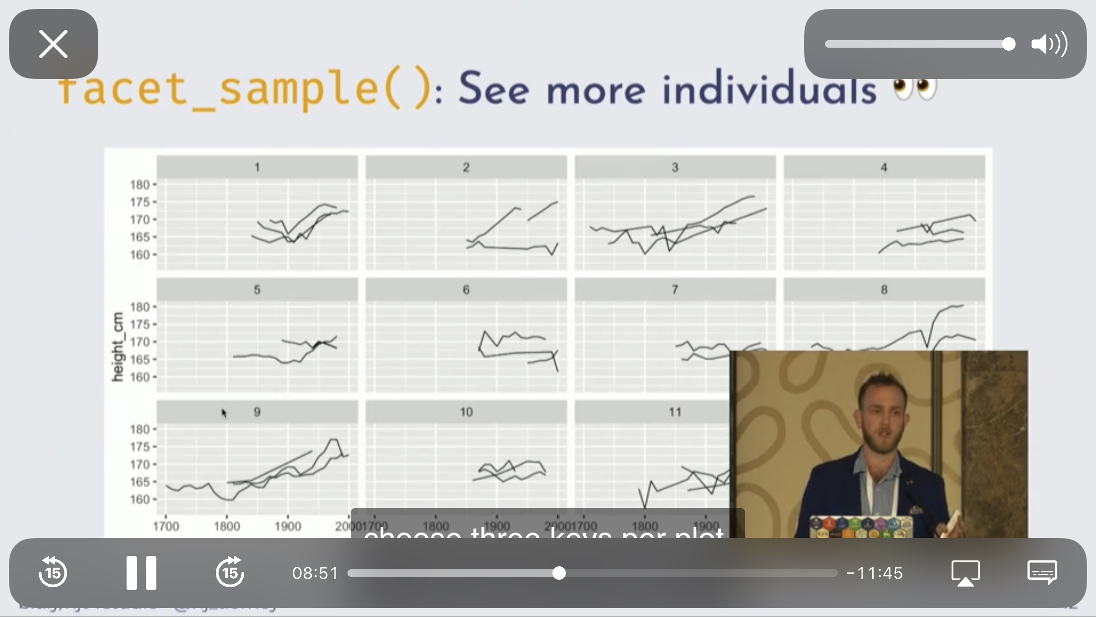
Figure 1.2: 可以考虑使用 ggplot2 来展示,一个 facet 展示至多3条线。一个图最好三个类别,这样可以减少读者的分心。(Tierney 2020)
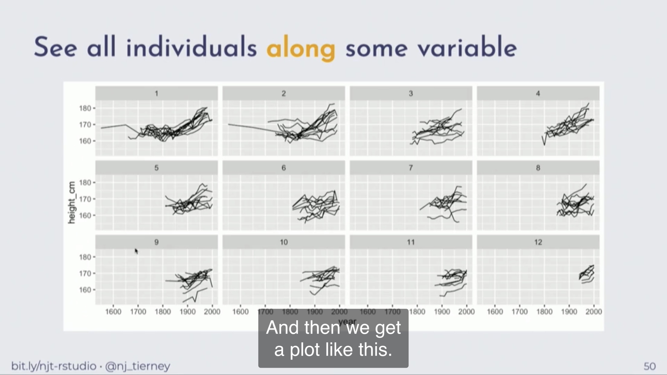
Figure 1.3: 按照顺序展示,如时间序列的长度,可以更加整齐一些。(Tierney 2020)
2 面板数据特殊性
##
## Attaching package: 'nlme'
## The following object is masked from 'package:glue':
##
## collapse## The following object is masked from 'package:dplyr':
##
## collapseggplot(BodyWeight, aes(x = factor(Time), y = weight)) +
geom_violin(aes(fill = Diet)) +
xlab("Time (in days)") +
ylab("Weight") +
theme_bw(base_size = 16)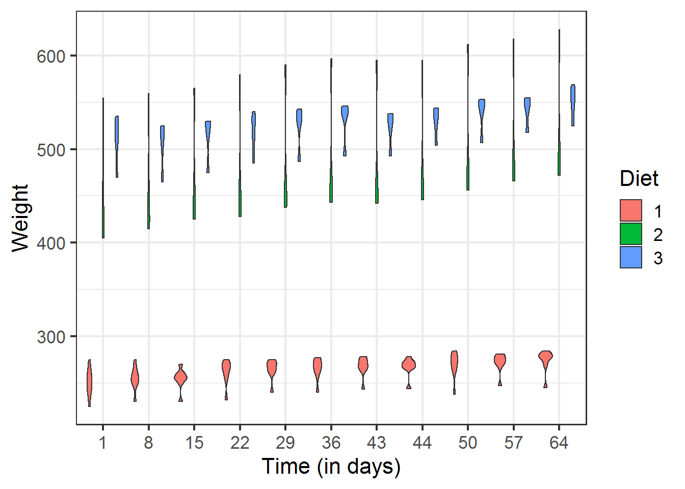
如图,我们发现不同组Diet之间 Weight 差异很大,而且是随着 Time 是相对稳定的。
但是我们是无法直接得到的,我们定义为 unobs effect 不可观测效应,图中显示的是固定效应,这就是其中一种。
(LeBeau 2019)
我们发现这种数据既然是在时间上保持稳定的,那么通过简单加减可以剔除,即使我们无法直接计算得到这种效应是多少。 这种处理方式产生了经济学里面固定效应模型。
3 Pooling 模型
平衡的面板数据是由多个相同长度的时间序列组成,我们知道单独分别做 OLS 回归,每个 beta 和截距肯定不同,但是 pooling 模型的目的是给出一个代表总体的方程,也就是混合回归(陈强 2019),这个已经给出了统一的方程为了还要训练固定效应模型呢?因为会产生辛普森悖论。
3.1 固定效应的剔除
- the between or inter-individual variability, which is the variability of panel’s variables measured in individual means, which is \(\overline{\boldsymbol{Z}}_{\boldsymbol{n}}\)
- the within or intra-individual variability, which is the variability of panel’s variables measured in deviation from individual means, which is \(z_{n t}-\overline{z}_{n}\)
一个特征变量组,其中的方差可以分为两部分,组间差异 (between) 和组内差异 (within),这两个英文词汇也非常直译。 组内差异就是我们常说的固定效应。
对于一个 Pooling 问题,可以分为三种处理方式
Three estimations by ordinary least squares can then be performed: the first one on raw data, the second one on the individual means of the data (between model), and the last one on the deviations from individual means (within model)
- 直接用原数据,也就是 pooling
- 用每个组的平均值,也就是 between
- 用每个组和组内均值差异,也就是 within。
其中可以介绍下他们的数学变换。
between 变换。
\[B=\mathrm{I}_{N} \otimes J_{T} / T\]
- \(J_{l}=j_{l} \times j_{l}^{\top}\)
- \(j_{l}\) 是单向量
举例 \(N=2 \text { 和 } T=3\)
\[B=\left(\begin{array}{cc}{1} & {0} \\ {0} & {1}\end{array}\right) \otimes\left[\left(\begin{array}{l}{1} \\ {1} \\ {1}\end{array}\right)\left(\begin{array}{lll}{1} & {1} & {1}\end{array}\right) / 3\right]\] \[=\left(\begin{array}{cc}{1} & {0} \\ {0} & {1}\end{array}\right) \otimes\left(\begin{array}{ccc}{1 / 3} & {1 / 3} & {1 / 3} \\ {1 / 3} & {1 / 3} & {1 / 3} \\ {1 / 3} & {1 / 3} & {1 / 3}\end{array}\right)\] \[=\left(\begin{array}{cccccc}{1 / 3} & {1 / 3} & {1 / 3} & {0} & {0} & {0} \\ {1 / 3} & {1 / 3} & {1 / 3} & {0} & {0} & {0} \\ {1 / 3} & {1 / 3} & {1 / 3} & {0} & {0} & {0} \\ {0} & {0} & {0} & {1 / 3} & {1 / 3} & {1 / 3} \\ {0} & {0} & {0} & {1 / 3} & {1 / 3} & {1 / 3} \\ {0} & {0} & {0} & {1 / 3} & {1 / 3} & {1 / 3}\end{array}\right)\]
因此
\[(B x)^{\top}=\left(\overline{x}_{1}, \overline{x}_{1}, \ldots, \overline{x}_{1}, \overline{x}_{2}, \overline{x}_{2}, \ldots, \overline{x}_{2}, \ldots, \overline{x}_{N,}, \overline{x}_{N .}, \ldots, \overline{x}_{N .}\right)\]
那么 within 变换为
\[W=\mathrm{I}_{N T}-\mathrm{I}_{N} \otimes J_{T} / T=\mathrm{I}_{N T}-B\]
这个推导很有意义。
那么进行 Within 变换时,产生以下等价关系
\[WX = (\mathrm{I}_{N T}-B)X = X - BX = X - \left(\overline{x}_{1}, \overline{x}_{1}, \ldots, \overline{x}_{1}, \overline{x}_{2}, \overline{x}_{2}, \ldots, \overline{x}_{2}, \ldots, \overline{x}_{N,}, \overline{x}_{N .}, \ldots, \overline{x}_{N .}\right)\]
因此各个变量都变成了组内均值为0的变量。那么一个 OLS 回归截距在什么时候成立呢?
\[y = \beta_0 + \beta_1 x + \mu\]
必然满足
\[\bar y = \beta_0 + \beta_1 \bar x + \bar \mu\] \[0 = \beta_0 + \beta_1 0 + 0\]
截距必然是0,以下举例,加以说明。
library(plm)
library(tidyverse)
data("TobinQ", package = "pder")
df <- TobinQ %>% select(cusip, year, ikn, qn)
df <-
df %>%
    group_by(cusip) %>%
    mutate_at(vars(ikn, qn), ~ . - mean(.))
df %>%
    group_by(cusip) %>%
summarise_at(vars(ikn, qn), mean)##
## Call:
## lm(formula = ikn ~ qn, data = df)
##
## Residuals:
## Min 1Q Median 3Q Max
## -0.21631 -0.04525 -0.00849 0.03365 0.61844
##
## Coefficients:
## Estimate Std. Error t value Pr(>|t|)
## (Intercept) 2.274e-18 8.874e-04 0.00 1
## qn 3.792e-03 1.702e-04 22.28 <2e-16 ***
## ---
## Signif. codes: 0 '***' 0.001 '**' 0.01 '*' 0.05 '.' 0.1 ' ' 1
##
## Residual standard error: 0.07198 on 6578 degrees of freedom
## Multiple R-squared: 0.07019, Adjusted R-squared: 0.07004
## F-statistic: 496.5 on 1 and 6578 DF, p-value: < 2.2e-16(Intercept) 趋近于0。beta1 的结果和 update(Q.pooling, model = "within") 相同,这是固定效应模型最直观的理解。
如果数学推导不是很好懂,可以看以下举例。
library(plm)
data("TobinQ", package = "pder")
pTobinQ <- pdata.frame(TobinQ)
pTobinQa <- pdata.frame(TobinQ, index = 188)
pTobinQb <- pdata.frame(TobinQ, index = c('cusip'))
pTobinQc <- pdata.frame(TobinQ, index = c('cusip', 'year'))
Qeq <- ikn ~ qn
Q.ols <- lm(Qeq, pTobinQ)
Q.pooling <- plm(Qeq, pTobinQ, model = "pooling")
Q.within <- update(Q.pooling, model = "within")
Q.between <- update(Q.pooling, model = "between")##
## =========================================================================================================================
## Dependent variable:
## -----------------------------------------------------------------------------------------------------
## ikn
## OLS panel
## linear
## (1) (2) (3) (4)
## -------------------------------------------------------------------------------------------------------------------------
## qn 0.004*** 0.004*** 0.004*** 0.005***
## (0.0002) (0.0002) (0.0002) (0.001)
##
## Constant 0.158*** 0.158*** 0.156***
## (0.001) (0.001) (0.004)
##
## -------------------------------------------------------------------------------------------------------------------------
## Observations 6,580 6,580 6,580 188
## R2 0.111 0.111 0.070 0.205
## Adjusted R2 0.111 0.111 0.043 0.201
## Residual Std. Error 0.086 (df = 6578)
## F Statistic 824.663*** (df = 1; 6578) 824.663*** (df = 1; 6578) 482.412*** (df = 1; 6391) 47.908*** (df = 1; 186)
## =========================================================================================================================
## Note: *p<0.1; **p<0.05; ***p<0.01within 情况,因为截距是常数,被剔除了。
The within model is also called the “fixed-effects model” or the least-squares dummy variable model, because it can be obtained as a linear model in which the individual effects are estimated and then taken as fixed parameters.
within 模型其实也叫做固定效应模型。
\[y=X \beta+\left(\mathrm{I}_{N} \otimes j_{T}\right) \eta+v\]
where \(\eta\) is now a vector of parameters to be estimated. Tere are therefore N + K parameters to estimate in this model. The \(N\) individual effects and the intercept \(\alpha\) can’t both be identified. Te choice made here consists in setting \(\alpha\)to 0.
因此 within 模型中,最后可以估计出每一个个体的个体效应(固定效应)。
3.2 固定效应的定义
The error component model is relevant when the slopes, i.e., the marginal effects of the covari ates on the response, are the same for all the individuals.
\[y_{n t}=\alpha+x_{n t}^{\top} \beta+\epsilon_{n t}\] \[\gamma^{\top}=\left(\alpha, \beta^{\top}\right)\] \[z_{n t}^{\top}=\left(1, x_{n t}^{\top}\right)\]
因此可以表示为
\[y_{n t}=z_{n t}^{\top} \gamma+\epsilon_{n t}\]
\[\epsilon_{n t}=\eta_{n}+v_{n t}\]
- 第一部分是个体效应
- 第二部分是异质效应
假设这里有 N 个个体,T 个时间,K 个变量 x 的长度为 \(N T \times K\)。
面板数据兼具了时间序列和截面数据的特性,因此也兼具两种数据产生的问题。因此需要做下面两种重要检验
- 相对于截面数据的,截面相依性
- 相对于时间序列的,单位根检验
3.3 固定效应检验
参考 Croissant and Millo (2018 Chapter 4.1)
3.3.1 F 检验
## Warning in pdata.frame(RiceFarms, index = "id"): column 'time' overwritten by
## time index
rice.w <-
plm(log(goutput) ~ log(seed) + log(totlabor) + log(size), Rice, model = "within")
rice.p <- update(rice.w, model = "pooling")
rice.wd <-
plm(log(goutput) ~ log(seed) + log(totlabor) + log(size),
Rice,
effect = "twoways")测试个体效应
##
##  F test for individual effects
##
## data:  log(goutput) ~ log(seed) + log(totlabor) + log(size)
## F = 1.6623, df1 = 170, df2 = 852, p-value = 2.786e-06
## alternative hypothesis: significant effects
术语可以不是模型的对象,也可以是表达式,
##
##  F test for individual effects
##
## data:  log(goutput) ~ log(seed) + log(totlabor) + log(size)
## F = 1.6623, df1 = 170, df2 = 852, p-value = 2.786e-06
## alternative hypothesis: significant effects
测试个体和时间固定效应
individual and time effects,
##
##  F test for twoways effects
##
## data:  log(goutput) ~ log(seed) + log(totlabor) + log(size)
## F = 4.2604, df1 = 175, df2 = 847, p-value < 2.2e-16
## alternative hypothesis: significant effects##
## F test for twoways effects
##
## data: log(goutput) ~ log(seed) + log(totlabor) + log(size)
## F = 4.2604, df1 = 175, df2 = 847, p-value < 2.2e-16
## alternative hypothesis: significant effects只测试时间固定效应
##
##  F test for twoways effects
##
## data:  log(goutput) ~ log(seed) + log(totlabor) + log(size)
## F = 69.779, df1 = 5, df2 = 847, p-value < 2.2e-16
## alternative hypothesis: significant effects
3.3.2 BP 检验
BP 检验是 Baltagi, Chang, and Li (1992) 提出,后面 King and Wu (1997) 和 Gouriéroux, Holly, and Monfort (1982) 也产生了变形。
##
##  Lagrange Multiplier Test - (Honda) for balanced panels
##
## data:  log(goutput) ~ log(seed) + log(totlabor) + log(size)
## normal = 4.8396, p-value = 6.507e-07
## alternative hypothesis: significant effects##
## Lagrange Multiplier Test - time effects (Honda) for balanced panels
##
## data: log(goutput) ~ log(seed) + log(totlabor) + log(size)
## normal = 58.682, p-value < 2.2e-16
## alternative hypothesis: significant effects##
## Lagrange Multiplier Test - two-ways effects (Honda) for balanced
## panels
##
## data: log(goutput) ~ log(seed) + log(totlabor) + log(size)
## normal = 44.917, p-value < 2.2e-16
## alternative hypothesis: significant effects##
## Lagrange Multiplier Test - (King and Wu) for balanced panels
##
## data: log(goutput) ~ log(seed) + log(totlabor) + log(size)
## normal = 4.8396, p-value = 6.507e-07
## alternative hypothesis: significant effects##
## Lagrange Multiplier Test - time effects (King and Wu) for balanced
## panels
##
## data: log(goutput) ~ log(seed) + log(totlabor) + log(size)
## normal = 58.682, p-value < 2.2e-16
## alternative hypothesis: significant effects##
## Lagrange Multiplier Test - two-ways effects (King and Wu) for balanced
## panels
##
## data: log(goutput) ~ log(seed) + log(totlabor) + log(size)
## normal = 58.656, p-value < 2.2e-16
## alternative hypothesis: significant effects##
## Lagrange Multiplier Test - (King and Wu) for balanced panels
##
## data: log(goutput) ~ log(seed) + log(totlabor) + log(size)
## normal = 4.8396, p-value = 6.507e-07
## alternative hypothesis: significant effects##
## Lagrange Multiplier Test - time effects (King and Wu) for balanced
## panels
##
## data: log(goutput) ~ log(seed) + log(totlabor) + log(size)
## normal = 58.682, p-value < 2.2e-16
## alternative hypothesis: significant effects##
## Lagrange Multiplier Test - two-ways effects (King and Wu) for balanced
## panels
##
## data: log(goutput) ~ log(seed) + log(totlabor) + log(size)
## normal = 58.656, p-value < 2.2e-16
## alternative hypothesis: significant effects4 单位根检验
read_lines("unit-root-test-learning-notes.Rmd") %>%
    str_replace("^(#+)\\s", "\\1# ") %>%
write_lines("unit-root-test-learning-notes-export.Rmd")- 使用 RMarkdown 的
child参数,进行文档拼接。 - 这样拼接以后的笔记方便复习。
- 相关问题提交到 GitHub
参考 Croissant and Millo (2018)
4.1 为什么要做单位根检验
\[y_{t}=\rho y_{t-1}+z_{t}^{\top} \gamma+\epsilon_{t}\]
如果 \(\rho = 1\) 那么产生了单位根。
下面举例介绍产生单位根的弊端。
## {
##     e <- rnorm(T)
##     for (t in 2:(T)) e[t] <- e[t] + rho * e[t - 1]
##     e
## }## {
## y <- autoreg(rho, T)
## x <- autoreg(rho, T)
## z <- lm(y ~ x) %>% broom::tidy()
## return(z)
## }run_on_test <- function(rho = 1, fun = tstat, T = 40, beta = 'x') {
beta1_df <-
data.frame(round = 1:1000) %>%
mutate(beta = map(round, ~ fun(rho = rho, T = T))) %>%
unnest() %>%
filter(term == beta)
beta1_df %>%
summarise(mean(abs(statistic) > 2)) %>%
print
beta1_df %>%
ggplot(aes(statistic)) +
geom_histogram()
}
run_on_test(rho = 0.2)## Warning: `cols` is now required.
## Please use `cols = c(beta)`## # A tibble: 1 x 1
## `mean(abs(statistic) > 2)`
## <dbl>
## 1 0.073## `stat_bin()` using `bins = 30`. Pick better value with `binwidth`.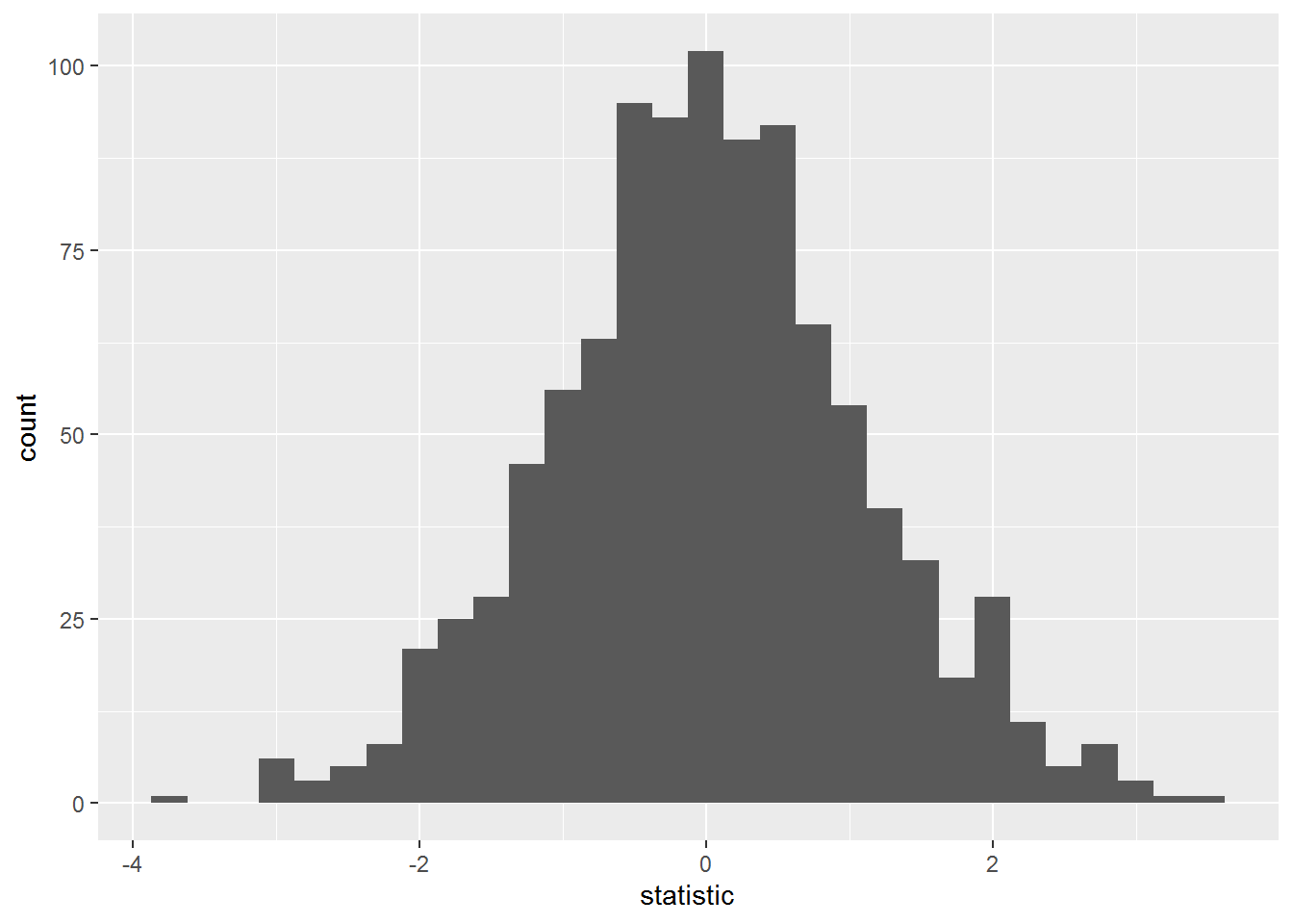
很明显,y 和 x 是分别单独构建的,因此之间相关性为0,因此 \(\beta_1=0\) 不能拒绝,我们计算出 t 值显著的情况(>2)在5%左右。我们只有 0.073 的概率拒绝原假设,因此很置信。
下面测试 \(\rho = 1\) 的情况。
## Warning: `cols` is now required.
## Please use `cols = c(beta)`
## # A tibble: 1 x 1
## `mean(abs(statistic) > 2)`
## <dbl>
## 1 0.62## `stat_bin()` using `bins = 30`. Pick better value with `binwidth`.
显然概率就大了很多,我们计算出 t 值显著的情况(>2)在远远大于5%,
我们有 0.62 的概率拒绝原假设,因此认为 x 是一个显著因子。
这就证明 y 和 x 相关性不为0,产生了伪回归 (spurious regression),给予我们 spurious 的显著因子。
4.2 发源
因此我们知道 \(\rho < 1\) 才能不出现伪回归,我们可以将之前的方程简化成,利用 OLS 回归进行检验。
\[\Delta y_{t}=(\rho-1) y_{t-1}+\epsilon_{t}\]
\[\mathrm{H}_{0} : \rho=1 , \mathrm{H}_{1} : \rho<1\]
source(here::here("R/autoreg.R"))
df_test <- function(rho = 0.2, T = 100) {
y <- autoreg(rho = rho, T = T)
Ly <- y[1:(T - 1)]
Dy <- y[2:T] - Ly
z <- lm(Dy ~ Ly)
broom::tidy(z)
}## Warning: `cols` is now required.
## Please use `cols = c(beta)`## # A tibble: 1 x 1
## `mean(abs(statistic) > 2)`
## <dbl>
## 1 1## `stat_bin()` using `bins = 30`. Pick better value with `binwidth`.
## Warning: `cols` is now required.
## Please use `cols = c(beta)`
## # A tibble: 1 x 1
## `mean(abs(statistic) > 2)`
## <dbl>
## 1 0.299## `stat_bin()` using `bins = 30`. Pick better value with `binwidth`.
- \(\rho = 0.2\) 有100%的情况拒绝原假设,不等于1
- \(\rho = 1\) 有70%的情况不能拒绝原假设
这就是 Dickey-Fuller 检验,在检验单位根时,是有效的。
4.3 co-integration 情况
这里说一种特殊情况,
\[y=\alpha+\beta x+\epsilon\]
如果 y 和 x 都有单位根,但是 \(\epsilon\) 没有,那么也可以说
they present a long-term structural relationship. One speaks then of co-integration.
y 和 x 有长期的结构关系,也可以说不是伪回归。
一般对 y ~ x 然后对 \(\epsilon\) 进行 DF 检验看是否有单位根。
参考 https://blog.csdn.net/FrankieHello/article/details/86770852
这里解释下单位根检验和协整检验 (co-integration) 的目的。 一般来说,我们不会拿到的数据都是平稳的 stationary,因此就是我们直接跑了 VAR,审稿人也不会相信。 因此我们会先把各个变量的单位根检验给出,如果发现不平稳的,一阶差分,查看是否平稳,一般假设是\((\rho-1)\)是否显著,显著了 \(\rho \neq 1\)。 但是我们做了一阶差分,那么差分后的变量就要去做 VAR,跑完以后要看看是否存在共线性的情况,如果存在,那么误差项就是不平稳的,也不行。因此需要对研究的方程做协整检验,目的是能够得到协整关系才行,也就是误差项是平稳的。否则我们 fit 的 VAR 也可能是伪回归。
这个地方可以注意到,协整的关系不一定要两个单变量的一元方程,可以放多个,参考 statsmodels.tsa.stattools.coint 的 help 文档,
y1 : array_like, 1d
    first element in cointegrating vector
y2 : array_like
    remaining elements in cointegrating vector
从展示角度,协整检验的结果还要展示方程,这里展示下 y1 和 y2 即可。
The Null hypothesis is that there is no cointegration, the alternativ hypothesis is that there is cointegrating relationship. If the pvalue is small, below a critical size, then we can reject the hypothesis that there is no cointegrating relationship.
我们需要协整关系存在,因此统计结果需要显著。
4.4 普通面板单位根检验
大多数单位根检验都是根据 DF 检验衍生的,最相近的是 augmented Dickey-Fuller 检验,简称 ADF 检验。
\[\Delta y_{n t}=\left(\rho_{n}-1\right) y_{n(t-1)}+\sum_{s=1}^{L_{n}} \theta_{n s} \Delta y_{n(t-s)}+\alpha_{m n}^{\top} d_{m t} \quad m=1,2,3\]
其中 \(d_{1 t}=\emptyset, d_{2 t}=1, d_{3 t}=1\)衡量截距和时间趋势。
\[\hat{\sigma}_{\epsilon_{n}}^{2}=\frac{\sum_{t=L_{n}+1}^{T} \hat{\epsilon}_{n t}^{2}}{d f_{n}}\]
这是残差方差估计。
因此产生了两个面板单位根检验。
Levin-Lin-Chu 检验是基于 ADF 检验产生的。
\[\Delta y_{n t} \sim \Delta y_{n t-s} s=1, \ldots L_{n}, d_{m t}\] \[y_{n t-1} \sim \Delta y_{n t-s} s=1, \ldots L_{n}, d_{m t}\]
然后得到分别残差项目 \(z_{n t}\) 和 \(\nu_{n(t-1)}\)
然后进行回归
\[z_{n t} / \hat{\sigma}_{n} \sim \nu_{n t} / \hat{\sigma}_{n}\]
查看 t 值是否显著。
One of the drawbacks of the Levin et al. (2002) test is that the alternative hypothesis holds that \(\rho \neq 1\) but at the same time it is the same for all individuals.
这是这个检验的缺点,没有考虑面板情况,因此备择假设是所有的个体都不存在单位根,这个假设过强,我们更需要的是,只要个体不全都有单位根就好了。
Im, Pesaran and Shin Test 是基于这个想法产生的。
对每个个体进行单位根检验,然后进行算数平均 \(\overline{t}=\frac{1}{N} \sum_{n=1}^{n} t_{\rho n}\)
The Maddala and Wu Test 也是基于这个想法产生的,只不过不是针对 t 值,而是 p 值,\(\mathrm{P}=-2 \sum_{n=1}^{N} \ln \mathrm{p}-\text { value }_{n}\)
library(plm)
data("HousePricesUS", package = "pder")
price <- pdata.frame(HousePricesUS)$price
purtest(log(price), test = "levinlin", lags = 2, exo = "trend")
##
## Levin-Lin-Chu Unit-Root Test (ex. var.: Individual Intercepts and
## Trend)
##
## data: log(price)
## z = -1.2573, p-value = 0.1043
## alternative hypothesis: stationarity##
## Maddala-Wu Unit-Root Test (ex. var.: Individual Intercepts and Trend)
##
## data: log(price)
## chisq = 99.843, df = 98, p-value = 0.4292
## alternative hypothesis: stationarity##
## Im-Pesaran-Shin Unit-Root Test (ex. var.: Individual Intercepts and
## Trend)
##
## data: log(price)
## Wtbar = 0.76622, p-value = 0.7782
## alternative hypothesis: stationarity我的建议是都把几种单位根检验结果做出,查看是否都支持结论。
4.5 和截面相依性的关系
Tis result depends on an assumption of cross-sectional independence. It is weakened if the errors are cross-sectionally weakly correlated, for example if they follow a spatial process, and can be expected to fail in presence of strong cross-sectional dependence, as would arise when omitting to control for common factors (Phillips and Moon, 1999, pages 1091–1092). Both pooled ols (Phillips and Sul, 2003) and mean groups estimators (Coakley et al., 2006) lose their advantage in precision from pooling when cross-sectional dependence is present.
因此在面板单位根检验前需要检验截面相依性。
4.6 鲁棒面板单位根检验
之前的面板单位根检验都没有考虑截面相依性,是用时间序列的思路去做面板单位根检验。 因此产生了 CADF 检验 (cross-sectionally augmented adf)。
\[\begin{aligned} \Delta y_{n t}=&\left(\rho_{n}-1\right) y_{n(t-1)}+\sum_{s=1}^{L_{n}} \theta_{n s} \Delta y_{n(t-s)}+\theta_{(s+1)} \overline{\Delta y}_{t}+\theta_{(s+2)} \overline{y}_{(t-1)} \\ &+\sum_{s=L_{n}+3}^{2 L_{n}+2} \theta_{s} \Delta y_{(t-s)}+\alpha_{m n}^{\top} d_{m t}(m=1,2,3) \end{aligned}\]
显然查看下角标,这里出现了 n 和 t 两个下角标。 但是正如前面的面板单位根检验,我们发现备择假设有两种,个体都没有单位根,个体不全有单位根。 在后面的 CADF 检验中,也会出现多种情况,例如 p-series 和其方程残差的的 CADF 检验是不一致的。
tab5a <- matrix(NA, ncol = 4, nrow = 2)
tab5b <- matrix(NA, ncol = 4, nrow = 2)
data("HousePricesUS", package = "pder")
for (i in 1:4) {
mymod <- pmg(
# Mean Groups (MG), Demeaned MG (DMG) and Common Correlated Effects MG (CCEMG) estimators for
# heterogeneous panel models, possibly with common factors (CCEMG)
diff(log(income)) ~ lag(log(income)) +
lag(diff(log(income)), 1:i),
data = HousePricesUS,
model = "mg",
trend = TRUE
)
tab5a[1, i] <- pcdtest(mymod, test = "rho")$statistic
tab5b[1, i] <- pcdtest(mymod, test = "cd")$statistic
}
for (i in 1:4) {
mymod <- pmg(
diff(log(price)) ~ lag(log(price)) +
lag(diff(log(price)), 1:i),
data = HousePricesUS,
model = "mg",
trend = TRUE
)
tab5a[2, i] <- pcdtest(mymod, test = "rho")$statistic
tab5b[2, i] <- pcdtest(mymod, test = "cd")$statistic
}
tab5a <- round(tab5a, 3)
tab5b <- round(tab5b, 2)
dimnames(tab5a) <- list(c("income", "price"),
paste("ADF(", 1:4, ")", sep = ""))
dimnames(tab5b) <- dimnames(tab5a)
tab5a## ADF(1) ADF(2) ADF(3) ADF(4)
## income 0.465 0.443 0.338 0.317
## price 0.346 0.326 0.252 0.194## ADF(1) ADF(2) ADF(3) ADF(4)
## income 82.84 77.40 57.96 53.21
## price 61.73 57.02 43.21 32.52显然,随着 AR 项目的增加,截面相依性下降。
## Warning in cipstest(log(php$price), type = "drift"): p-value greater than
## printed p-value
##
## Pesaran's CIPS test for unit roots
##
## data: log(php$price)
## CIPS test = -2.0342, lag order = 2, p-value = 0.1
## alternative hypothesis: Stationarity## Warning in cipstest(diff(log(php$price)), type = "none"): p-value smaller than
## printed p-value##
## Pesaran's CIPS test for unit roots
##
## data: diff(log(php$price))
## CIPS test = -1.8199, lag order = 2, p-value = 0.01
## alternative hypothesis: Stationarity显然这里显示 log(php$price 是有单位根,但是一阶差分是没有的。
##
##  Pesaran's CIPS test for unit roots
##
## data:  log(php$income)
## CIPS test = -2.1503, lag order = 2, p-value = 0.0383
## alternative hypothesis: Stationarity
ccemgmod <- pcce(log(price) ~ log(income), data=HousePricesUS, model="mg")
ccepmod <- pcce(log(price) ~ log(income), data=HousePricesUS, model="p")## Warning in cipstest(resid(ccemgmod), type = "none"): p-value smaller than
## printed p-value##
## Pesaran's CIPS test for unit roots
##
## data: resid(ccemgmod)
## CIPS test = -2.6588, lag order = 2, p-value = 0.01
## alternative hypothesis: Stationarity## Warning in cipstest(resid(ccepmod), type = "none"): p-value smaller than printed
## p-value##
## Pesaran's CIPS test for unit roots
##
## data: resid(ccepmod)
## CIPS test = -2.2395, lag order = 2, p-value = 0.01
## alternative hypothesis: Stationarity可以看出目前两个模型都没有单位根,那么 log(price) 和 log(income) 是 co-integrated 的,结论是可信的。
5 截面相依性检验
read_lines("cross-sectional-dependence-learning-notes.Rmd") %>%
    str_replace("^(#+)\\s", "\\1# ") %>%
write_lines("cross-sectional-dependence-learning-notes-export.Rmd")- 使用 RMarkdown 的
child参数,进行文档拼接。 - 这样拼接以后的笔记方便复习。
- 相关问题提交到 GitHub
参考 Croissant and Millo (2018)
5.1 截面相依性定义
If cross-sectional dependence is present, the consequence is, at a minimum, inefficiency of the usual estimators and invalid inference when using the standard covariance matrix. Tis is the case, for example, in unobserved effects models when cross-sectional dependence is due to an unobservable factor structure but with factors uncorrelated with the regressors. In this case the within or re are still consistent, although inefficient (see De Hoyos and Sarafidis, 2006). If the unobserved factors are correlated with the regressors, which can seldom be ruled out, consequences are more serious: the estimators will be inconsistent.
截面相依性的存在会让模型估计的标准协方差矩阵失效。
- 如果不可观察效应和自变量不相关时,
within和RE模型还是一致的,但是不是有效的。 - 如果不可观察效应和自变量相关时,模型将会不一致。
一致和有效是面板模型最主要的两个指标,因此需要在模型进行前,进行检验。
一般来说,检验的指标计算过程如下。
\[\text{Pairwise Correlation Coefficients} = \hat{\rho}_{n m}=\frac{\sum_{t=1}^{T} \hat{z}_{n t} \hat{z}_{m t}}{\left(\sum_{t=1}^{T} \hat{z}_{n t}^{2}\right)^{1 / 2}\left(\sum_{t=1}^{T} \hat{z}_{m t}^{2}\right)^{1 / 2}}\]
这里查看的两两个不同 id 之间的相关系数。 这里一共产生了 \(N(N-1)\) 个相关系数,汇总为
\[\hat{\rho}=1 /(N(N-1)) \sum_{n=1}^{N} \sum_{m=1}^{n-1} \hat{\rho}_{n m}\] \[\hat{\rho}_{\mathrm{ABS}}=1 /(N(N-1)) \sum_{n=1}^{N} \sum_{m=1}^{n-1}\left|\hat{\rho}_{n m}\right|\]
使用\(\hat{\rho}_{\mathrm{ABS}}\)是为了防止 \(\hat{\rho}_{n m}\) 正负抵消。
plm::pcdtest 函数基本上都是基于这两个指标进行线性变换计算的。
Breusch-Pagan LM test,适用于 N 小 T 大的情况
\[\mathrm{LM}_{\rho}=\sum_{n=1}^{N-1} \sum_{m=n+1}^{N} T_{n m} \hat{\rho}_{n m}^{2}\]
5.2 检验代码
Pairwise-correlations-based tests are originally meant to use the residuals of separate esti mation of one time-series regression for each cross-sectional unit.
一般来说这里的相关系数是针对模型残差的。
以下举例。
##
## Breusch-Pagan LM test for cross-sectional dependence in panels
##
## data: lny ~ lnl + lnk + lnrd
## chisq = 12134, df = 7021, p-value < 2.2e-16
## alternative hypothesis: cross-sectional dependence##
## Pesaran CD test for cross-sectional dependence in panels
##
## data: lny ~ lnl + lnk + lnrd
## z = 28.612, p-value < 2.2e-16
## alternative hypothesis: cross-sectional dependence使用 CD test 需要注意的地方。
The test is compatible with any consistent plm model for the data at hand, with any specification of effect; e.g., specifying
effect = ’time’oreffect = ’twoways’allows to test for residual cross-sectional dependence after the introduction of time fixed effects to account for common shocks.
这里使用 CD test 时需要注意,
\[\mathbf{CD}=\sqrt{\frac{2}{N(N-1)}}\left(\sum_{n=1}^{N-1} \sum_{m=n+1}^{N} \sqrt{T_{n m}} \hat{\rho}_{n m}\right)\]
\(\hat{\rho}_{n m}\) 可正可负,因此 CD 等于 0,并不代表不含有截面相依性。
##
## Pesaran CD test for cross-sectional dependence in panels
##
## data: lny ~ lnl + lnk + lnrd
## z = -1.4637, p-value = 0.1433
## alternative hypothesis: cross-sectional dependence##
## Average correlation coefficient for cross-sectional dependence in
## panels
##
## data: lny ~ lnl + lnk + lnrd
## rho = -0.0048794
## alternative hypothesis: cross-sectional dependence##
## Average absolute correlation coefficient for cross-sectional
## dependence in panels
##
## data: lny ~ lnl + lnk + lnrd
## |rho| = 0.50209
## alternative hypothesis: cross-sectional dependence##
## Breusch-Pagan LM test for cross-sectional dependence in panels
##
## data: lny ~ lnl + lnk + lnrd
## chisq = 44732, df = 7021, p-value < 2.2e-16
## alternative hypothesis: cross-sectional dependence##
## Pesaran CD test for cross-sectional dependence in panels
##
## data: lny ~ lnl + lnk + lnrd
## z = -1.4637, p-value = 0.1433
## alternative hypothesis: cross-sectional dependence我们发现使用 \(\hat{\rho}_{\mathbf{A B S}}\) 计量后,截面相依性还是很强的。
总结上,因此当发现没有截面相依性时,多做几种测试查看。
5.3 对变量进行检验
5.3.1 静态
tests in the cd family can be employed in preliminary statistical assessments as well, in order to determine whether the dependent and explanatory variables show any correlation to begin with.
之前测试的是残差的截面相依性,以下测试因变量或者自变量是否有截面相依性。
##
## Breusch-Pagan LM test for cross-sectional dependence in panels
##
## data: diff(log(php$price))
## chisq = 7993.9, df = 1176, p-value < 2.2e-16
## alternative hypothesis: cross-sectional dependence##
## Pesaran CD test for cross-sectional dependence in panels
##
## data: diff(log(php$price))
## z = 72.802, p-value < 2.2e-16
## alternative hypothesis: cross-sectional dependence## rho
## 0.3942212## |rho|
## 0.4246933检验得知,截面相依性很强。
regions.names <- c(
"New Engl",
"Mideast",
"Southeast",
"Great Lks",
"Plains",
"Southwest",
"Rocky Mnt",
"Far West"
)
corr.table.hp <- plm:::cortab(diff(log(php$price)),
grouping = php$region,
groupnames = regions.names)
colnames(corr.table.hp) <- substr(rownames(corr.table.hp), 1, 5)
round(corr.table.hp, 2)## New E Midea South Great Plain South Rocky Far W
## New Engl 0.80 NA NA NA NA NA NA NA
## Mideast 0.68 0.66 NA NA NA NA NA NA
## Southeast 0.40 0.35 0.81 NA NA NA NA NA
## Great Lks 0.27 0.20 0.62 0.61 NA NA NA NA
## Plains 0.40 0.32 0.57 0.53 0.52 NA NA NA
## Southwest 0.07 -0.05 0.28 0.39 0.35 0.52 NA NA
## Rocky Mnt -0.03 -0.11 0.52 0.53 0.40 0.57 0.70 NA
## Far West 0.13 0.17 0.52 0.42 0.29 0.31 0.46 0.57这里可以发现一些地区是正相关的、一些地区是负相关的,这是截面相依性最直观的表现。
5.3.2 动态
the properties of the CD test rest on the hypothesis of no serial correlation, we follow Pesaran (2004)’s suggestion to remove any by specifying a univariate ar(2) model of the variable of interest and proceed testing the residuals of the latter for cross-sectional dependence.
CD 这个检验显然必须满足没有时间自相关性。因此在控制变量中加入 y 的滞后项,例如控制 AR(2) 来达到效果。
##
## Pesaran CD test for cross-sectional dependence in panels
##
## data: diff(log(price)) ~ diff(lag(log(price))) + diff(lag(log(price), 2))
## z = 59.009, p-value < 2.2e-16
## alternative hypothesis: cross-sectional dependence5.4 附录
5.4.1 OLS 右偏证明
参考 econpapers
\[y_{i t}=\mathbf{x}_{i t}^{\prime} \boldsymbol{\theta}_{i}+u_{i t}, i=1,2, \ldots, N, t=1,2, \ldots, T\]
假设面板数据满足上述回归方程, 其中 \(\mathbf{x}_{i t}\)包含截距和\(y_{i t}\)的滞后项等。
同时我们假设\(y_{i t}\)是通过以下方程模拟出来的。
\[y_{i t}=\mathbf{x}_{i t}^{\prime} \boldsymbol{\beta}_{i}+\mathbf{z}_{t}^{\prime} \boldsymbol{\gamma}_{i}+\varepsilon_{i t}\]
\(\mathbf{z}_{t}\)衡量我们无法观测的效应,并且在不同 id 之间都相关,因此固定效应模型无法单纯去除,这就是截面相依性。
同时\(\mathbf{x}_{i t}\)和\(\mathbf{z}_{i t}\)两者可相关,因此产生方程
\[\mathbf{z}_{t}^{\prime}=\mathbf{x}_{i t}^{\prime} \mathbf{D}_{i}+\boldsymbol{\eta}_{i t}^{\prime}\]
已知\(\mathbf{z}_{t}\)衡量我们无法观测的效应,并且在不同 id 之间都相关,那么这个效应不会是\(\mathbf{x}_{i t}\)表现,而是\(\boldsymbol{\eta}_{i t}^{\prime}\),因此它衡量了截面相依性。
我们将上述方程整理后得到
\[y_{i t}=\mathbf{x}_{i t}^{\prime}\left(\boldsymbol{\beta}_{i}+\mathbf{D}_{i} \gamma_{i}\right)+\boldsymbol{\eta}_{i t}^{\prime} \boldsymbol{\gamma}_{i}+\varepsilon_{i t}\]
然后我们从 OLS 回归的角度讨论 \(u_{i t}\)
\[u_{i t}=\boldsymbol{\eta}_{i t}^{\prime} \boldsymbol{\gamma}_{i}+\varepsilon_{i t}=\mathbf{z}_{t}^{\prime} \boldsymbol{\gamma}_{i}-\mathbf{x}_{i t}^{\prime} \mathbf{D}_{i} \boldsymbol{\gamma}_{i}+\varepsilon_{i t}\]
我们发现\(u_{i t}\)和\(\boldsymbol{\eta}_{i t}\)相关,因此截面相依性会导致 OLS 假设不满足,产生有偏估计。
6 异回归系数问题
6.1 介绍
我们在 3 了解到,都是不同国家、组用一个回归系数估计,不考虑国家之间的差异,这样显然在时间序列很长的情况下不满足。这一章节主要讲这部分问题。
Panel time series methods were born to address the issues of “long” panels of possibly non- stationary series, usually of macroeconomic nature. Such datasets, pooling together a sizable number of time series from different countries (regions, firms) have become increasingly common and are the main object of empirical research in many fields
这类定义名称叫做 panel time series,是 long panels,也定义了是 several 国家。
The assumption of parameter homogeneity is also often questioned in this field, often leading to relaxing it in favor of heterogeneous specifications where the coefficients of individual units are free to vary over the cross-section. The parameter of interest can then be either the whole population of individual ones or the cross-sectional average thereof.
对于面板时间序列,再用一个方程的参数衡量所有国家就不适用了,因此每个个体的参数都可以变动。
\[y_{n t}=\eta_{n}+\rho y_{n t-1}+\beta x_{n t}+v_{n t}\]
如这个动态残差模型。
\(\eta_{n}\) 和 \(x_{n t}\) 相关。当 \(T \rightarrow \infty\) 模型的偏差下降,模型是一致的。
we know that the within estimator for this model is in turn biased downward, the bias being inversely proportional to T so that it becomes less severe as the available time dimension gets longer.
当 T 增加时,OLS 回归的偏误下降。以下解释。
From a different viewpoint, if each time series in the panel is considered separately, as \(T \rightarrow \infty\), ols are a consistent estimator for the individual parameters \(\left(\rho_{n}, \beta_{n}\right)\) so that sepa- rately estimating, and then either averaging or pooling, the coefficients becomes a feasible strategy.
这种理解是更直接的,为什么 T 增加,OLS 估计更准。
如果 T 很大,那么模型的常数和分别执行多个 OLS 回归差异不大,因此可以直接执行 Pooling 的方程。
where the long time dimension allows to address unit roots and cointegration; and cross-sectional dependence across individual units, possibly due to common factors to which individual units react idiosyncratically
因此 long time panels 可以解决很多检验暴露的问题。
Long panels allow to estimate separate regressions for each unit. Hence it is natural to question the assumption of parameter homogeneity (\(\beta_{n}=\beta \forall n\), also called the pooling assumption) as opposed to various kinds of heterogeneous specifications.
这点我也统一,当是好几个长时间序列时,假设都是同一个 beta 的意义就不大了。
This is a vast subject, which we will keep as simple as possible here; in general it can be said that imposing the pooling restriction reduces the variance of the pooled estimator but may introduce bias if these restrictions are false (Baltagi et al., 2008). Moreover, the heterogeneous model is usually a generalization of the homogeneous one so that estimating it may allow to test for the validity of the pooling restriction.
也就是说 poolling 的假设是不一定满足的。
\[y_{n t}=\alpha+\beta_{n} x_{n t}+\eta_{n}+v_{n t}\]
因此 \(\beta_{n}\) 对于每一个个体都有。 \(\beta_{n}\)代表了 n 组自变量。
6.2 固定效应
\[y_{n t}=\alpha+\beta_{n} x_{n t}+\eta_{n}+v_{n t}\]
直接估计每个的 \(\hat{\beta}_{\mathrm{ous}, n}=\left(X_{n}^{\top} X_{n}\right)^{-1} X_{n}^{\top} y_{n}\) 即可。
但是显然参数很多,是 \(NK\) 个参数。因此一般不适用,因此随机效应会更好些。
6.3 随机效应
Swamy 估计
\[y_{n t}=\gamma_{n}^{\top} z_{n t}+v_{n t}\]
- \(\gamma_{n} \sim N(\gamma, \Delta), \text { or } \delta_{n}=\gamma_{n}-\gamma \sim N(0, \Delta)\)
\[y_{n t}=\gamma^{\top} z_{n t}+\epsilon_{n t} \quad \epsilon_{n t}=v_{n t}+\delta_{n}^{\top} z_{n t}\]
简言之,pooling 的参数 \(\gamma^{\top\) 相当于每个个体参数的正态分布均值,\(\gamma_{n}^{\top\) 围绕其波动。
data("Dialysis", package = "pder")
rndcoef <- pvcm(log(diffusion / (1 - diffusion)) ̃ trend + trend:regulation,
Dialysis, model="random")
summary(rndcoef)
Oneway (individual) effect Random coefficients model
Call:
pvcm(formula = log(diffusion/(1 - diffusion)) ̃ trend + trend:regulation,
data = Dialysis, model = "random")
Balanced Panel: n = 50, T = 14, N = 700
Residuals:
total sum of squares: 629.5
id time
0.4685 0.2659
Estimated mean of the coefficients:
Estimate Std. Error z-value Pr(>|z|)
(Intercept) -1.4266 0.1284 -11.11 <2e-16 ***
trend 0.3416 0.0260 13.15 <2e-16 ***
trend:regulation -0.0581 0.0237 -2.45 0.014 *
---
Signif. codes:
0 '***' 0.001 '**' 0.01 '*' 0.05 '.' 0.1 ' ' 1
Estimated variance of the coefficients:
(Intercept) trend trend:regulation
(Intercept) 0.6617 -0.0736 0.0398
trend -0.0736 0.0288 -0.0205
trend:regulation 0.0398 -0.0205 0.0179
Total Sum of Squares: 33900
Residual Sum of Squares: 642
Multiple R-Squared: 0.981cbind(coef(rndcoef), stdev = sqrt(diag(rndcoef$Delta)))
y stdev
(Intercept) -1.42656 0.8135
trend 0.34161 0.1697
trend:regulation -0.05806 0.1339The random coefficients have large standard deviations: about half the mean for the trend coefficient and about two times the mean for the regulation coefficients. These large values justify the use of the random coefficient model.
因此个体之间的差异很大,不能假设每个个体效应都是一个常数。
6.4 平均组模型
基于 Swamy 估计上更简单的开发。
assuming only exogeneity of the regressors and independently sampled errors, the average \(\gamma\) can be estimated.
因此这里的自变量内不加入 y 变量的滞后一期。
估计非常简单
\[\hat{\gamma}_{\mathrm{MG}}=\frac{1}{N} \sum_{n=1}^{N} \hat{\gamma}_{\mathrm{ous}, n}\]
因此方差为
\[V\left(\hat{\gamma}_{\mathrm{MG}}\right)=\frac{1}{N(N-1)} \sum_{n=1}^{N}\left(\hat{\gamma}_{\mathrm{ous}, n}-\hat{\gamma}_{\mathrm{MG}}\right)\left(\hat{\gamma}_{\mathrm{ous}, n}-\hat{\gamma}_{\mathrm{MG}}\right)^{\top}\]
data("HousePricesUS", package = "pder")
swmod <-
pvcm(log(price) ~ log(income), data = HousePricesUS, model = "random")
mgmod <-
pmg(log(price) ~ log(income), data = HousePricesUS, model = "mg")
coefs <- cbind(coef(swmod), coef(mgmod))
dimnames(coefs)[[2]] <- c("Swamy", "MG")
coefs## Swamy MG
## (Intercept) 3.8914242 3.8498054
## log(income) 0.2867014 0.3018117One can see that for \(T = 29\), the efficient Swamy estimator and the simpler mg are already very close; moreover, both are statistically very far from one.
\(T = 29\) 结果就已经非常接近了,因此不需要 Swamy 估计那么严格。
下面考虑动态情况,Dynamic Mean Groups。
\[y_{n t}=\rho_{n} y_{n t-1}+\gamma_{n}^{\top} z_{n t}+v_{n t}\]
\(\rho_{n}\) 也是对应了不同个体。
library("texreg")
data("RDSpillovers", package = "pder")
fm.rds <- lny ~ lnl + lnk + lnrd
mg.rds <- pmg(fm.rds, RDSpillovers, trend = TRUE)
dmg.rds <- update(mg.rds, . ~ lag(lny) + .)
screenreg(list('Static MG' = mg.rds, 'Dynamic MG' = dmg.rds), digits = 3)##
## =======================================
## Static MG Dynamic MG
## ---------------------------------------
## (Intercept) 4.550 *** 4.038 ***
## (0.841) (0.778)
## lnl 0.568 *** 0.507 ***
## (0.086) (0.059)
## lnk 0.117 0.020
## (0.122) (0.085)
## lnrd -0.058 -0.092
## (0.079) (0.071)
## trend 0.022 ** 0.023 ***
## (0.008) (0.004)
## lag(lny) 0.223 ***
## (0.034)
## ---------------------------------------
## Num. obs. 2637 2518
## =======================================
## *** p < 0.001, ** p < 0.01, * p < 0.05显然这个数据集中,lag(lny) 是非常显著的。
6.5 Pooling 检验
显然目前我们知道可以 poolling 也可以对各个个体进行估计。那么什么时候使用前者,什么时候使用后者,也有对应的检验。
对应地,我们使用 Chow 检验,检验两个模型的差异,可以使用 plm::pooltest 估计。
\[\frac{\hat{\epsilon}_{\mathrm{w}}^{\top} \hat{\epsilon}_{\mathrm{w}}-\hat{\epsilon}_{n p}^{\top} \hat{\epsilon}_{n p}}{\hat{\epsilon}_{n p}^{\top} \hat{\epsilon}_{n p}} \frac{N(T-K-1)}{(N-1) K}\]
housep.np <- pvcm(log(price) ~  log(income), data = HousePricesUS,
                  model = "within")
housep.pool <- plm(log(price) ~  log(income), data = HousePricesUS,
                   model = "pooling")
housep.within <- plm(log(price) ~  log(income), data = HousePricesUS,
model = "within")##
## F statistic
##
## data: log(price) ~ log(income)
## F = 25.778, df1 = 96, df2 = 1323, p-value < 2.2e-16
## alternative hypothesis: unstability##
## F statistic
##
## data: log(price) ~ log(income)
## F = 16.074, df1 = 48, df2 = 1323, p-value < 2.2e-16
## alternative hypothesis: unstabilitydepending on whether we want to assume absence of individual effects or not.
这里就看我们能不能简化的使用 pooling 即可。
Coefficient stability is very strongly rejected, even in its weakest form (specific constants).
查看这里的 p 值 和 H1,pooling 估计是不稳定的,因此需要使用我们讨论的考虑个体情况的模型。
6.6 Pooled Mean Group 模型
PMG 模型理论推导超出这里 intro 水平,感兴趣可以查看 8.1,但是比较好理解的是,它会把一个研究变量对被解释变量的边际效应,区分长短期的情况。这是我们之前模型没有讨论到的创新点。下面会以一个例子来解释。
6.6.1 实现例子
这个例子采集自 cran,其中变量的解释可以参考自它。
source(here::here("../imp_rmd/R/load.R"))
library(PooledMeanGroup)
# first import DataExp, i=1...9, T1=T2=...T9=35
data("DataExp", package = "PooledMeanGroup")
DataExp[1:5, ]
# then prepare lags and diffs using LagPanel and DiffPanel
y10 = data.frame(y10 = DataExp[, 1], row.names = row.names(DataExp))
cpi = data.frame(cpi = DataExp[, 7], row.names = row.names(DataExp))
dy10 = DiffPanel(variable = y10, quantity = rep(35, 9))
dopeness = DiffPanel(variable = DataExp[, 6], quantity = rep(35, 9))
ly10 = LagPanel(variable = y10, quantity = rep(35, 9))
diip = DiffPanel(variable = DataExp[, 11], quantity = rep(35, 9))
dcrisk = DiffPanel(variable = DataExp[, 9], quantity = rep(35, 9))
ldcrisk = LagPanel(variable = dcrisk, quantity = rep(35, 9))
dcpi = DiffPanel(variable = DataExp[, 7], quantity = rep(35, 9))
ddcpi = DiffPanel(variable = dcpi, quantity = rep(35, 9))
ldebt = LagPanel(variable = DataExp[, 4], quantity = rep(35, 9))Zientara and Kujawski (2017) 采用的示例数据,如下。
df_keys <- rownames(DataExp) %>% str_split(",", n = 3, simplify = TRUE) %>% as.data.frame() %>%
`names<-`(c("id", "t", "qt"))
df_keys %>%
print()## id t qt
## 1 i=1 t=1 2005q2
## 2 i=1 t=2 2005q3
## 3 i=1 t=3 2005q4
## 4 i=1 t=4 2006q1
## 5 i=1 t=5 2006q2
## 6 i=1 t=6 2006q3
## 7 i=1 t=7 2006q4
## 8 i=1 t=8 2007q1
## 9 i=1 t=9 2007q2
## 10 i=1 t=10 2007q3
## 11 i=1 t=11 2007q4
## 12 i=1 t=12 2008q1
## 13 i=1 t=13 2008q2
## 14 i=1 t=14 2008q3
## 15 i=1 t=15 2008q4
## 16 i=1 t=16 2009q1
## 17 i=1 t=17 2009q2
## 18 i=1 t=18 2009q3
## 19 i=1 t=19 2009q4
## 20 i=1 t=20 2010q1
## 21 i=1 t=21 2010q2
## 22 i=1 t=22 2010q3
## 23 i=1 t=23 2010q4
## 24 i=1 t=24 2011q1
## 25 i=1 t=25 2011q2
## 26 i=1 t=26 2011q3
## 27 i=1 t=27 2011q4
## 28 i=1 t=28 2012q1
## 29 i=1 t=29 2012q2
## 30 i=1 t=30 2012q3
## 31 i=1 t=31 2012q4
## 32 i=1 t=32 2013q1
## 33 i=1 t=33 2013q2
## 34 i=1 t=34 2013q3
## 35 i=1 t=35 2013q4
## 36 i=2 t=1 2005q2
## 37 i=2 t=2 2005q3
## 38 i=2 t=3 2005q4
## 39 i=2 t=4 2006q1
## 40 i=2 t=5 2006q2
## 41 i=2 t=6 2006q3
## 42 i=2 t=7 2006q4
## 43 i=2 t=8 2007q1
## 44 i=2 t=9 2007q2
## 45 i=2 t=10 2007q3
## 46 i=2 t=11 2007q4
## 47 i=2 t=12 2008q1
## 48 i=2 t=13 2008q2
## 49 i=2 t=14 2008q3
## 50 i=2 t=15 2008q4
## 51 i=2 t=16 2009q1
## 52 i=2 t=17 2009q2
## 53 i=2 t=18 2009q3
## 54 i=2 t=19 2009q4
## 55 i=2 t=20 2010q1
## 56 i=2 t=21 2010q2
## 57 i=2 t=22 2010q3
## 58 i=2 t=23 2010q4
## 59 i=2 t=24 2011q1
## 60 i=2 t=25 2011q2
## 61 i=2 t=26 2011q3
## 62 i=2 t=27 2011q4
## 63 i=2 t=28 2012q1
## 64 i=2 t=29 2012q2
## 65 i=2 t=30 2012q3
## 66 i=2 t=31 2012q4
## 67 i=2 t=32 2013q1
## 68 i=2 t=33 2013q2
## 69 i=2 t=34 2013q3
## 70 i=2 t=35 2013q4
## 71 i=3 t=1 2005q2
## 72 i=3 t=2 2005q3
## 73 i=3 t=3 2005q4
## 74 i=3 t=4 2006q1
## 75 i=3 t=5 2006q2
## 76 i=3 t=6 2006q3
## 77 i=3 t=7 2006q4
## 78 i=3 t=8 2007q1
## 79 i=3 t=9 2007q2
## 80 i=3 t=10 2007q3
## 81 i=3 t=11 2007q4
## 82 i=3 t=12 2008q1
## 83 i=3 t=13 2008q2
## 84 i=3 t=14 2008q3
## 85 i=3 t=15 2008q4
## 86 i=3 t=16 2009q1
## 87 i=3 t=17 2009q2
## 88 i=3 t=18 2009q3
## 89 i=3 t=19 2009q4
## 90 i=3 t=20 2010q1
## 91 i=3 t=21 2010q2
## 92 i=3 t=22 2010q3
## 93 i=3 t=23 2010q4
## 94 i=3 t=24 2011q1
## 95 i=3 t=25 2011q2
## 96 i=3 t=26 2011q3
## 97 i=3 t=27 2011q4
## 98 i=3 t=28 2012q1
## 99 i=3 t=29 2012q2
## 100 i=3 t=30 2012q3
## 101 i=3 t=31 2012q4
## 102 i=3 t=32 2013q1
## 103 i=3 t=33 2013q2
## 104 i=3 t=34 2013q3
## 105 i=3 t=35 2013q4
## 106 i=4 t=1 2005q2
## 107 i=4 t=2 2005q3
## 108 i=4 t=3 2005q4
## 109 i=4 t=4 2006q1
## 110 i=4 t=5 2006q2
## 111 i=4 t=6 2006q3
## 112 i=4 t=7 2006q4
## 113 i=4 t=8 2007q1
## 114 i=4 t=9 2007q2
## 115 i=4 t=10 2007q3
## 116 i=4 t=11 2007q4
## 117 i=4 t=12 2008q1
## 118 i=4 t=13 2008q2
## 119 i=4 t=14 2008q3
## 120 i=4 t=15 2008q4
## 121 i=4 t=16 2009q1
## 122 i=4 t=17 2009q2
## 123 i=4 t=18 2009q3
## 124 i=4 t=19 2009q4
## 125 i=4 t=20 2010q1
## 126 i=4 t=21 2010q2
## 127 i=4 t=22 2010q3
## 128 i=4 t=23 2010q4
## 129 i=4 t=24 2011q1
## 130 i=4 t=25 2011q2
## 131 i=4 t=26 2011q3
## 132 i=4 t=27 2011q4
## 133 i=4 t=28 2012q1
## 134 i=4 t=29 2012q2
## 135 i=4 t=30 2012q3
## 136 i=4 t=31 2012q4
## 137 i=4 t=32 2013q1
## 138 i=4 t=33 2013q2
## 139 i=4 t=34 2013q3
## 140 i=4 t=35 2013q4
## 141 i=5 t=1 2005q2
## 142 i=5 t=2 2005q3
## 143 i=5 t=3 2005q4
## 144 i=5 t=4 2006q1
## 145 i=5 t=5 2006q2
## 146 i=5 t=6 2006q3
## 147 i=5 t=7 2006q4
## 148 i=5 t=8 2007q1
## 149 i=5 t=9 2007q2
## 150 i=5 t=10 2007q3
## 151 i=5 t=11 2007q4
## 152 i=5 t=12 2008q1
## 153 i=5 t=13 2008q2
## 154 i=5 t=14 2008q3
## 155 i=5 t=15 2008q4
## 156 i=5 t=16 2009q1
## 157 i=5 t=17 2009q2
## 158 i=5 t=18 2009q3
## 159 i=5 t=19 2009q4
## 160 i=5 t=20 2010q1
## 161 i=5 t=21 2010q2
## 162 i=5 t=22 2010q3
## 163 i=5 t=23 2010q4
## 164 i=5 t=24 2011q1
## 165 i=5 t=25 2011q2
## 166 i=5 t=26 2011q3
## 167 i=5 t=27 2011q4
## 168 i=5 t=28 2012q1
## 169 i=5 t=29 2012q2
## 170 i=5 t=30 2012q3
## 171 i=5 t=31 2012q4
## 172 i=5 t=32 2013q1
## 173 i=5 t=33 2013q2
## 174 i=5 t=34 2013q3
## 175 i=5 t=35 2013q4
## 176 i=6 t=1 2005q2
## 177 i=6 t=2 2005q3
## 178 i=6 t=3 2005q4
## 179 i=6 t=4 2006q1
## 180 i=6 t=5 2006q2
## 181 i=6 t=6 2006q3
## 182 i=6 t=7 2006q4
## 183 i=6 t=8 2007q1
## 184 i=6 t=9 2007q2
## 185 i=6 t=10 2007q3
## 186 i=6 t=11 2007q4
## 187 i=6 t=12 2008q1
## 188 i=6 t=13 2008q2
## 189 i=6 t=14 2008q3
## 190 i=6 t=15 2008q4
## 191 i=6 t=16 2009q1
## 192 i=6 t=17 2009q2
## 193 i=6 t=18 2009q3
## 194 i=6 t=19 2009q4
## 195 i=6 t=20 2010q1
## 196 i=6 t=21 2010q2
## 197 i=6 t=22 2010q3
## 198 i=6 t=23 2010q4
## 199 i=6 t=24 2011q1
## 200 i=6 t=25 2011q2
## 201 i=6 t=26 2011q3
## 202 i=6 t=27 2011q4
## 203 i=6 t=28 2012q1
## 204 i=6 t=29 2012q2
## 205 i=6 t=30 2012q3
## 206 i=6 t=31 2012q4
## 207 i=6 t=32 2013q1
## 208 i=6 t=33 2013q2
## 209 i=6 t=34 2013q3
## 210 i=6 t=35 2013q4
## 211 i=7 t=1 2005q2
## 212 i=7 t=2 2005q3
## 213 i=7 t=3 2005q4
## 214 i=7 t=4 2006q1
## 215 i=7 t=5 2006q2
## 216 i=7 t=6 2006q3
## 217 i=7 t=7 2006q4
## 218 i=7 t=8 2007q1
## 219 i=7 t=9 2007q2
## 220 i=7 t=10 2007q3
## 221 i=7 t=11 2007q4
## 222 i=7 t=12 2008q1
## 223 i=7 t=13 2008q2
## 224 i=7 t=14 2008q3
## 225 i=7 t=15 2008q4
## 226 i=7 t=16 2009q1
## 227 i=7 t=17 2009q2
## 228 i=7 t=18 2009q3
## 229 i=7 t=19 2009q4
## 230 i=7 t=20 2010q1
## 231 i=7 t=21 2010q2
## 232 i=7 t=22 2010q3
## 233 i=7 t=23 2010q4
## 234 i=7 t=24 2011q1
## 235 i=7 t=25 2011q2
## 236 i=7 t=26 2011q3
## 237 i=7 t=27 2011q4
## 238 i=7 t=28 2012q1
## 239 i=7 t=29 2012q2
## 240 i=7 t=30 2012q3
## 241 i=7 t=31 2012q4
## 242 i=7 t=32 2013q1
## 243 i=7 t=33 2013q2
## 244 i=7 t=34 2013q3
## 245 i=7 t=35 2013q4
## 246 i=8 t=1 2005q2
## 247 i=8 t=2 2005q3
## 248 i=8 t=3 2005q4
## 249 i=8 t=4 2006q1
## 250 i=8 t=5 2006q2
## 251 i=8 t=6 2006q3
## 252 i=8 t=7 2006q4
## 253 i=8 t=8 2007q1
## 254 i=8 t=9 2007q2
## 255 i=8 t=10 2007q3
## 256 i=8 t=11 2007q4
## 257 i=8 t=12 2008q1
## 258 i=8 t=13 2008q2
## 259 i=8 t=14 2008q3
## 260 i=8 t=15 2008q4
## 261 i=8 t=16 2009q1
## 262 i=8 t=17 2009q2
## 263 i=8 t=18 2009q3
## 264 i=8 t=19 2009q4
## 265 i=8 t=20 2010q1
## 266 i=8 t=21 2010q2
## 267 i=8 t=22 2010q3
## 268 i=8 t=23 2010q4
## 269 i=8 t=24 2011q1
## 270 i=8 t=25 2011q2
## 271 i=8 t=26 2011q3
## 272 i=8 t=27 2011q4
## 273 i=8 t=28 2012q1
## 274 i=8 t=29 2012q2
## 275 i=8 t=30 2012q3
## 276 i=8 t=31 2012q4
## 277 i=8 t=32 2013q1
## 278 i=8 t=33 2013q2
## 279 i=8 t=34 2013q3
## 280 i=8 t=35 2013q4
## 281 i=9 t=1 2005q2
## 282 i=9 t=2 2005q3
## 283 i=9 t=3 2005q4
## 284 i=9 t=4 2006q1
## 285 i=9 t=5 2006q2
## 286 i=9 t=6 2006q3
## 287 i=9 t=7 2006q4
## 288 i=9 t=8 2007q1
## 289 i=9 t=9 2007q2
## 290 i=9 t=10 2007q3
## 291 i=9 t=11 2007q4
## 292 i=9 t=12 2008q1
## 293 i=9 t=13 2008q2
## 294 i=9 t=14 2008q3
## 295 i=9 t=15 2008q4
## 296 i=9 t=16 2009q1
## 297 i=9 t=17 2009q2
## 298 i=9 t=18 2009q3
## 299 i=9 t=19 2009q4
## 300 i=9 t=20 2010q1
## 301 i=9 t=21 2010q2
## 302 i=9 t=22 2010q3
## 303 i=9 t=23 2010q4
## 304 i=9 t=24 2011q1
## 305 i=9 t=25 2011q2
## 306 i=9 t=26 2011q3
## 307 i=9 t=27 2011q4
## 308 i=9 t=28 2012q1
## 309 i=9 t=29 2012q2
## 310 i=9 t=30 2012q3
## 311 i=9 t=31 2012q4
## 312 i=9 t=32 2013q1
## 313 i=9 t=33 2013q2
## 314 i=9 t=34 2013q3
## 315 i=9 t=35 2013q4因此我们发现这里 t 有 35 期,id 有 9 个,唯一值有 315,刚好等于 (\(35 \times 9\)),因此以下设定rep(35, 9))。
# create homogenous preliminary dataset (containing "NA" as a result of DiffPanel, LagPanel)
dataPanel = cbind(y10,
dy10,
ly10,
DataExp[, 6],
dopeness,
diip,
DataExp[, 11],
ldcrisk,
DataExp[, 9],
ddcpi,
DataExp[, 7])
dataPanel = data.frame(dataPanel)
names(dataPanel) = c(
"y10",
"dy10",
"ly10",
"openess",
"dopeness",
"diip",
"iip",
"ldcrisk",
"crisk",
"ddcpi",
"cpi"
)
dataPanel[1:5, ]# prepare dataset and quantity for PMG or optimPMG functions using PanelNaOmit
dataPanel = PanelNaOmit(dataset = dataPanel, quantity = rep(35, 9))
dataPanel$dataset[1:5, ]## [1] 33 33 33 33 33 33 33 33 33# PMG
PmgExp = PMG(
paramTeta = c(-14.22768,-23.84427,-0.75717, 27.57753),
vecSR = list(
SR1 = c("dy10", "dopeness", "diip", "ldcrisk", "ddcpi"),
SR2 = c("dy10", "dopeness", "diip", "ldcrisk", "ddcpi"),
SR3 = c("dy10", "dopeness", "diip", "ldcrisk", "ddcpi"),
SR4 = c("dy10", "dopeness", "diip", "ldcrisk", "ddcpi"),
SR5 = c("dy10", "dopeness", "diip", "ldcrisk", "ddcpi"),
SR6 = c("dy10", "dopeness", "diip", "ldcrisk", "ddcpi"),
SR7 = c("dy10", "dopeness", "diip", "ldcrisk", "ddcpi"),
SR8 = c("dy10", "dopeness", "diip", "ldcrisk", "ddcpi"),
SR9 = c("dy10", "dopeness", "diip", "ldcrisk", "ddcpi")
),
vecLR = c("ly10", "openess", "iip", "crisk", "cpi"),
dataset = dataPanel$dataset,
quantity = dataPanel$quantity,
const = TRUE
)Pooled Mean Group 模型还没有归纳到 plm 包内,但是可以通过 PooledMeanGroup 包实现其中的中间过程,最后进行简单运算计算出短期效应。
Pesaran, Shin, and Smith (1999) 在构建时,是可以算出每个个体的短期效应,但是大部分学者,如 Bangake and Eggoh (2012) 只会展示一个整体的短期效应。以下的将 PmgExp 的短期效应结果清洗为一个整体的短期效应。
Having particular long-run parameters (exp. start values) estimates parameters of short-run relationships as well as standard errors of estimations, Student’s t-distribution type statistics, probs, confidence intervals.
paramTeta = c(-14.22768,-23.84427,-0.75717, 27.57753), 表示长期均衡已经假定了。
## List of 9
## $ :'data.frame': 6 obs. of 6 variables:
## ..$ Coef(i=1): num [1:6] -0.0325 5.7814 -0.7155 -0.1129 10.2521 ...
## ..$ StdErr : num [1:6] 0.022 4.1053 0.9682 0.0593 5.6134 ...
## ..$ z : num [1:6] -1.477 1.408 -0.739 -1.903 1.826 ...
## ..$ P>|z| : num [1:6] 0.1398 0.1591 0.4599 0.057 0.0678 ...
## ..$ Low95% : num [1:6] -0.0757 -2.2649 -2.6131 -0.2291 -0.75 ...
## ..$ High95% : num [1:6] 0.01064 13.8277 1.18214 0.00338 21.25423 ...
## $ :'data.frame': 6 obs. of 6 variables:
## ..$ Coef(i=2): num [1:6] 0.00544 -0.10515 0.5249 -0.01504 -10.09013 ...
## ..$ StdErr : num [1:6] 0.0362 1.0657 1.8417 0.0862 5.0191 ...
## ..$ z : num [1:6] 0.1504 -0.0987 0.285 -0.1744 -2.0104 ...
## ..$ P>|z| : num [1:6] 0.8805 0.9214 0.7756 0.8615 0.0444 ...
## ..$ Low95% : num [1:6] -0.0654 -2.1938 -3.0847 -0.184 -19.9273 ...
## ..$ High95% : num [1:6] 0.0763 1.9836 4.1345 0.1539 -0.253 ...
## $ :'data.frame': 6 obs. of 6 variables:
## ..$ Coef(i=3): num [1:6] -0.0297 -3.237 1.6089 0.0488 3.7668 ...
## ..$ StdErr : num [1:6] 0.0318 2.9981 1.9867 0.0841 5.6981 ...
## ..$ z : num [1:6] -0.933 -1.08 0.81 0.58 0.661 ...
## ..$ P>|z| : num [1:6] 0.351 0.28 0.418 0.562 0.509 ...
## ..$ Low95% : num [1:6] -0.0921 -9.1132 -2.285 -0.116 -7.4013 ...
## ..$ High95% : num [1:6] 0.0327 2.6391 5.5028 0.2137 14.9349 ...
## $ :'data.frame': 6 obs. of 6 variables:
## ..$ Coef(i=4): num [1:6] -0.0123 -0.7727 -0.018 0.2405 11.3901 ...
## ..$ StdErr : num [1:6] 0.0077 3.3876 0.4756 0.1308 10.4563 ...
## ..$ z : num [1:6] -1.5922 -0.2281 -0.0379 1.8384 1.0893 ...
## ..$ P>|z| : num [1:6] 0.111 0.82 0.97 0.066 0.276 ...
## ..$ Low95% : num [1:6] -0.0274 -7.4123 -0.9502 -0.0159 -9.104 ...
## ..$ High95% : num [1:6] 0.00283 5.86696 0.91415 0.49682 31.88413 ...
## $ :'data.frame': 6 obs. of 6 variables:
## ..$ Coef(i=5): num [1:6] -0.10826 1.06266 0.09463 0.00282 -5.59085 ...
## ..$ StdErr : num [1:6] 0.0284 4.9234 1.4637 0.0775 8.6714 ...
## ..$ z : num [1:6] -3.8067 0.2158 0.0647 0.0363 -0.6447 ...
## ..$ P>|z| : num [1:6] 0.000141 0.829115 0.948449 0.971027 0.519093 ...
## ..$ Low95% : num [1:6] -0.164 -8.587 -2.774 -0.149 -22.587 ...
## ..$ High95% : num [1:6] -0.0525 10.7124 2.9634 0.1548 11.4049 ...
## $ :'data.frame': 6 obs. of 6 variables:
## ..$ Coef(i=6): num [1:6] -0.661 3.586 9.528 0.382 -7.995 ...
## ..$ StdErr : num [1:6] 0.109 2.837 4.255 0.166 11.449 ...
## ..$ z : num [1:6] -6.091 1.264 2.239 2.309 -0.698 ...
## ..$ P>|z| : num [1:6] 1.12e-09 2.06e-01 2.51e-02 2.10e-02 4.85e-01 ...
## ..$ Low95% : num [1:6] -0.8742 -1.975 1.1882 0.0578 -30.4347 ...
## ..$ High95% : num [1:6] -0.449 9.147 17.868 0.707 14.444 ...
## $ :'data.frame': 6 obs. of 6 variables:
## ..$ Coef(i=7): num [1:6] -0.119 5.357 2.333 -0.274 -9.149 ...
## ..$ StdErr : num [1:6] 0.0398 3.616 2.3734 0.1197 7.0229 ...
## ..$ z : num [1:6] -3.001 1.481 0.983 -2.289 -1.303 ...
## ..$ P>|z| : num [1:6] 0.00269 0.1385 0.32568 0.02206 0.19269 ...
## ..$ Low95% : num [1:6] -0.197 -1.73 -2.319 -0.509 -22.913 ...
## ..$ High95% : num [1:6] -0.0414 12.444 6.9845 -0.0394 4.6162 ...
## $ :'data.frame': 6 obs. of 6 variables:
## ..$ Coef(i=8): num [1:6] -0.0251 -1.2953 0.0137 -0.0416 3.5709 ...
## ..$ StdErr : num [1:6] 0.0206 1.4658 1.1897 0.0927 9.9138 ...
## ..$ z : num [1:6] -1.2192 -0.8837 0.0115 -0.4488 0.3602 ...
## ..$ P>|z| : num [1:6] 0.223 0.377 0.991 0.654 0.719 ...
## ..$ Low95% : num [1:6] -0.0655 -4.1682 -2.3181 -0.2232 -15.8598 ...
## ..$ High95% : num [1:6] 0.0153 1.5776 2.3455 0.14 23.0016 ...
## $ :'data.frame': 6 obs. of 6 variables:
## ..$ Coef(i=9): num [1:6] 0.00423 -1.46738 -1.28602 0.12845 10.99649 ...
## ..$ StdErr : num [1:6] 0.0429 2.9067 2.0444 0.0747 5.8332 ...
## ..$ z : num [1:6] 0.0986 -0.5048 -0.6291 1.7191 1.8852 ...
## ..$ P>|z| : num [1:6] 0.9215 0.6137 0.5293 0.0856 0.0594 ...
## ..$ Low95% : num [1:6] -0.0798 -7.1645 -5.2929 -0.018 -0.4363 ...
## ..$ High95% : num [1:6] 0.0882 4.2297 2.7209 0.2749 22.4293 ...PmgExp$SR2 <-
map(1:9, ~ PmgExp$SR %>% .[[.x]] %>% `names<-`(c("Coef", "StdErr", "z", "P>|z|", "Low95%", "High95%")) %>% rownames_to_column) %>%
bind_rows() %>%
group_by(rowname) %>%
summarise(
Coef = mean(Coef, na.rm = TRUE),
StdErr = sqrt(sum(StdErr^2, na.rm = TRUE)),
na_Coef = sum(is.na(Coef)),
na_StdErr = sum(is.na(StdErr))
) %>%
filter(!rowname %>% str_detect("^ec\\d"))\[\beta_{SR} = \frac{\sum_{1}^{N}\beta_{SR}^{i}}{N}\] \[\text{sd}_{SR} = \sqrt{\frac{\sum_{1}^{N}(\text{sd}_{SR}^{i})^2}{N}}\]
PmgExp$LR 表示长期效应,PmgExp$SR2 表示短期效应。
我们可以发下短期效应绝对值都是小于长期效应的,这可以让我们理解为长期效应是短期效应累计而得到的。
6.6.2 长期均衡获得方式
# then prepare lags and diffs using LagPanel and DiffPanel
y10 = data.frame(y10 = DataExp[, 1], row.names = row.names(DataExp))
cpi = data.frame(cpi = DataExp[, 7], row.names = row.names(DataExp))
dy10 = DiffPanel(variable = y10, quantity = rep(35, 9))
dopeness = DiffPanel(variable = DataExp[, 6], quantity = rep(35, 9))
ly10 = LagPanel(variable = y10, quantity = rep(35, 9))
diip = DiffPanel(variable = DataExp[, 11], quantity = rep(35, 9))
dcrisk = DiffPanel(variable = DataExp[, 9], quantity = rep(35, 9))
ldcrisk = LagPanel(variable = dcrisk, quantity = rep(35, 9))
dcpi = DiffPanel(variable = DataExp[, 7], quantity = rep(35, 9))
ddcpi = DiffPanel(variable = dcpi, quantity = rep(35, 9))
ldebt = LagPanel(variable = DataExp[, 4], quantity = rep(35, 9))
# create homogenous preliminary dataset (containing "NA" as a result of DiffPanel, LagPanel)
dataPanel = cbind(y10,
dy10,
ly10,
DataExp[, 6],
dopeness,
diip,
DataExp[, 11],
ldcrisk,
DataExp[, 9],
ddcpi,
DataExp[, 7])
dataPanel = data.frame(dataPanel)
names(dataPanel) = c(
"y10",
"dy10",
"ly10",
"openess",
"dopeness",
"diip",
"iip",
"ldcrisk",
"crisk",
"ddcpi",
"cpi"
)参考 Zientara and Kujawski (2017)
TetaStart = rep(x = 1, times = 4) 设定初始值都为1,然后迭代,类似于梯度下降 8.2 的进行方式。
# prepare dataset and quantity for PMG or optimPMG functions using PanelNaOmit
dataPanel = PanelNaOmit(dataset = dataPanel, quantity = rep(35, 9))
dataPanel$dataset[1:5, ]## [1] 33 33 33 33 33 33 33 33 33# optimPMG
OptimPmgExp = optimPMG(
dLL = 10 ^ -10,
maxIter = 200,
TetaStart = rep(x = 1, times = 4),
# note that length(TetaStart)=length(vecLR)-1
vecSR = list(
SR1 = c("dy10", "dopeness", "diip", "ldcrisk", "ddcpi"),
SR2 = c("dy10", "dopeness", "diip", "ldcrisk", "ddcpi"),
SR3 = c("dy10", "dopeness", "diip", "ldcrisk", "ddcpi"),
SR4 = c("dy10", "dopeness", "diip", "ldcrisk", "ddcpi"),
SR5 = c("dy10", "dopeness", "diip", "ldcrisk", "ddcpi"),
SR6 = c("dy10", "dopeness", "diip", "ldcrisk", "ddcpi"),
SR7 = c("dy10", "dopeness", "diip", "ldcrisk", "ddcpi"),
SR8 = c("dy10", "dopeness", "diip", "ldcrisk", "ddcpi"),
SR9 = c("dy10", "dopeness", "diip", "ldcrisk", "ddcpi")
),
vecLR = c("ly10", "openess", "iip", "crisk", "cpi"),
dataset = dataPanel$dataset,
quantity = dataPanel$quantity,
const = TRUE
)7 神经网络应用
7.1 数据处理
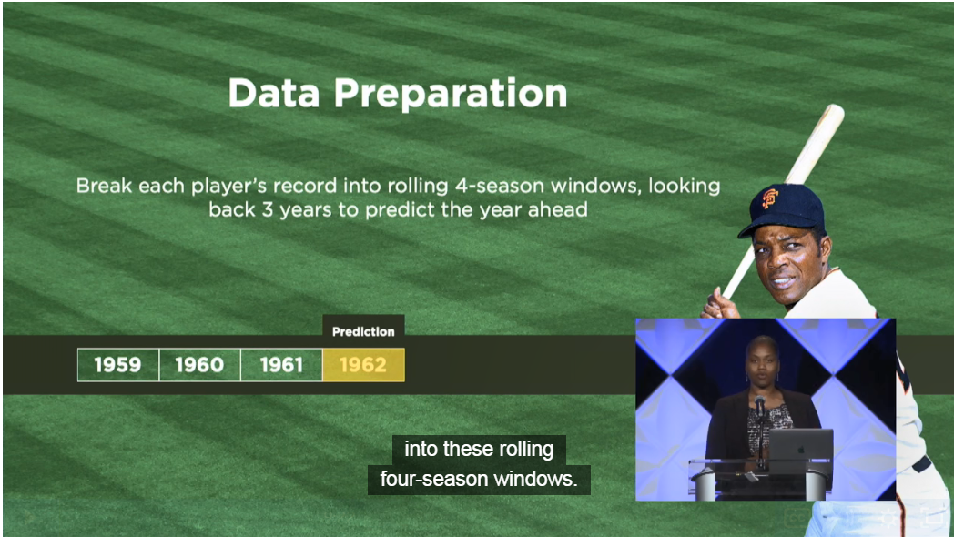
Figure 7.1: LSTM rolling windows 提取特征是一个常见的方法,这样按照4个单位为窗口长度,前三个作为特征,后一个作为 label。如果球员 skip 的赛季就 padding。
但是因为 LSTM 的结构,本身允许每个样本大小不一样,因此也可以把一个球员全部的赛季信息录入(Watson 2020),暂时无实验数据验证哪一种更好。
Data split 按照球员分,也就是说一个球员的数据只会在 train valid 和 test 中一个数据集中出现,防止信息漏出。
7.2 在 OLS、GBM的模型上进行比较
7.2.1 OLS
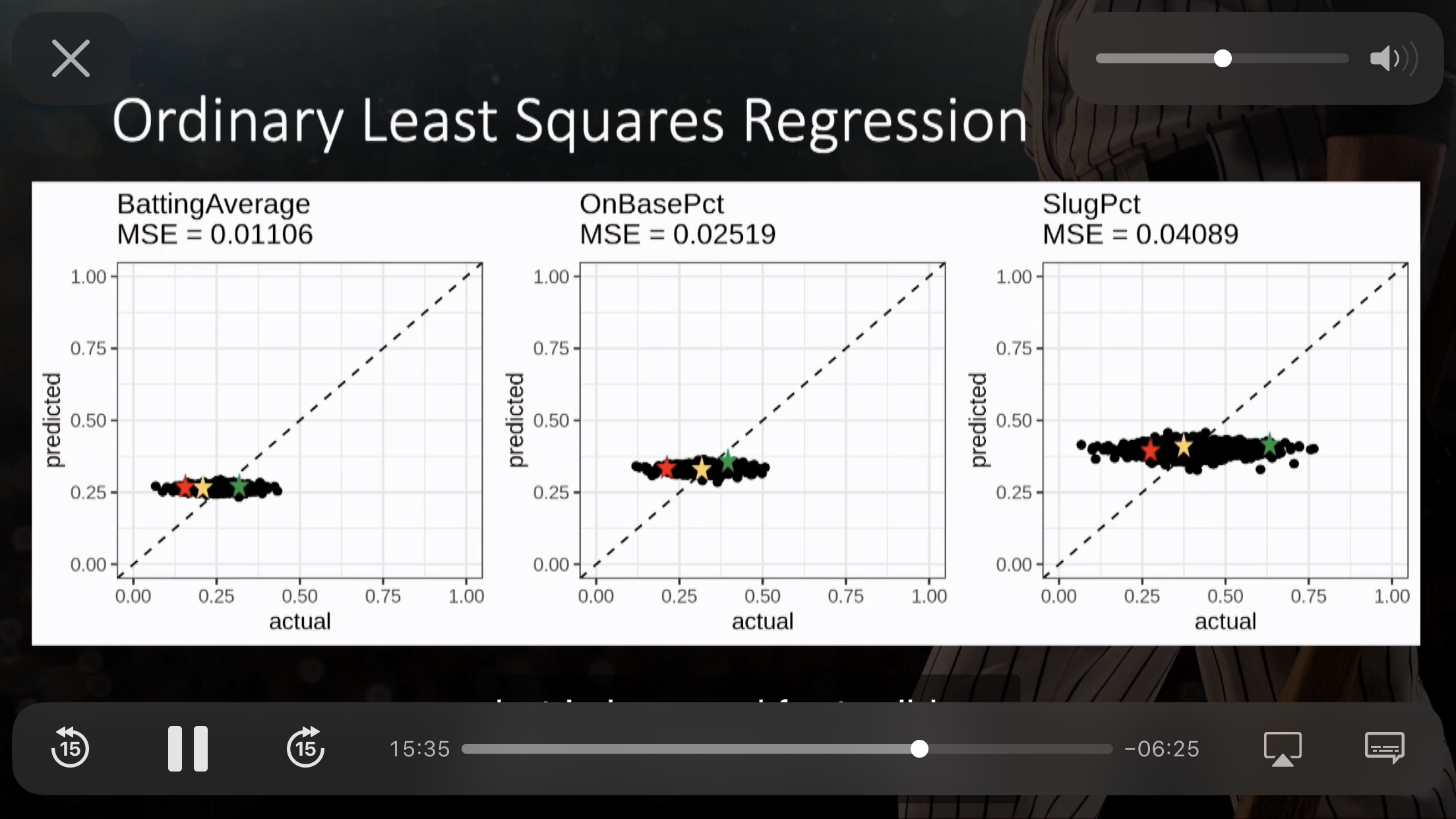
Figure 7.2: 见校正曲线,当预测值为某一个值的时候,真实值有很大的 range。(Watson 2020)
7.2.2 GBM
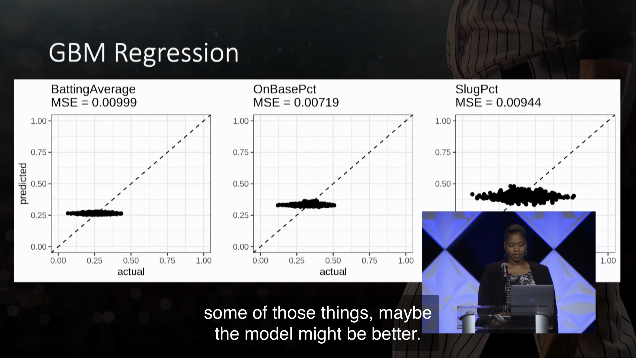
Figure 7.3: 见校正曲线,当预测值为某一个值的时候,真实值有很大的 range。(Watson 2020)
7.2.3 NN
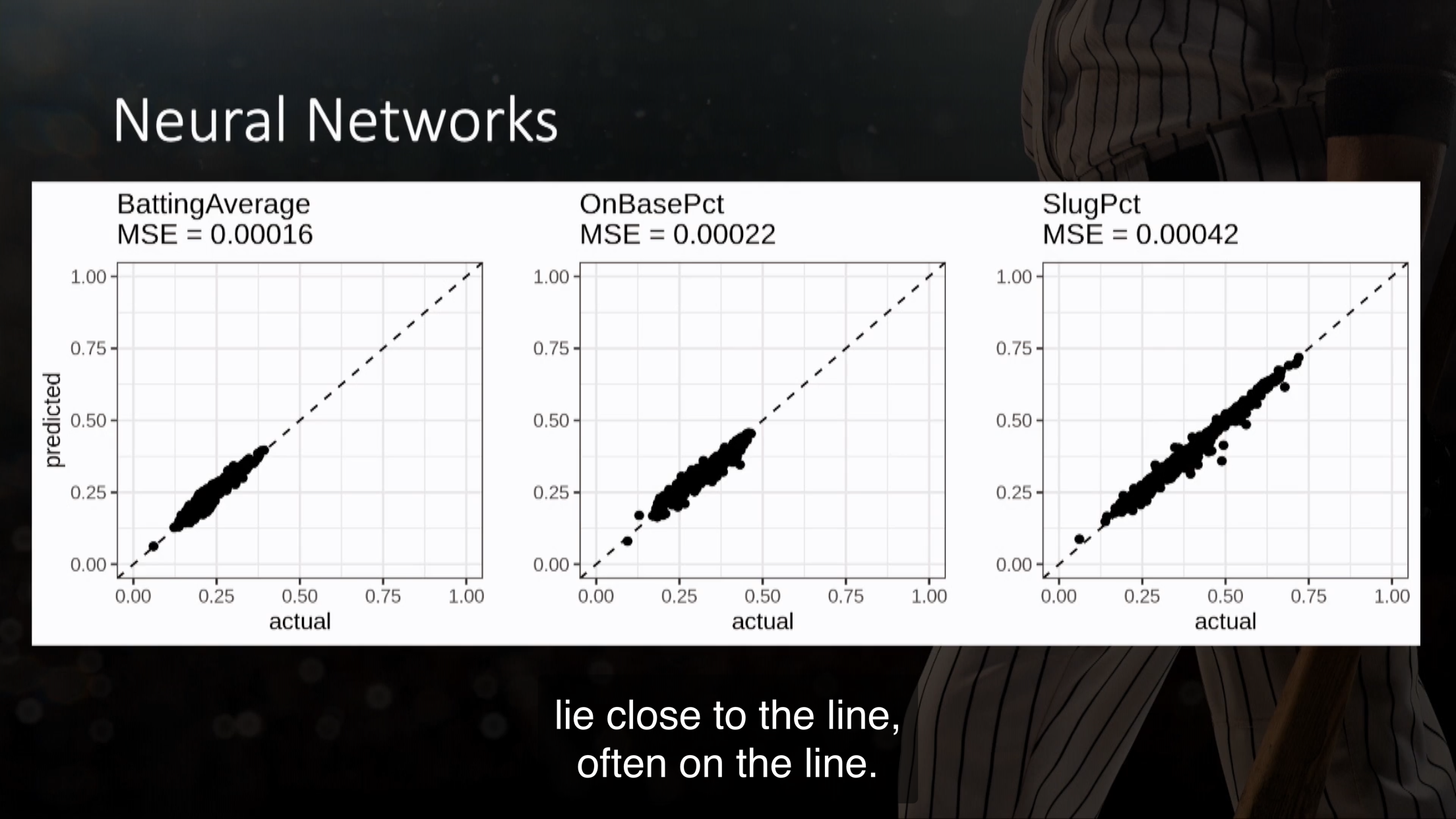
Figure 7.4: 见校正曲线,基本都在45度线上了。这个效果未免太好。(Watson 2020)
8 附录
8.1 PMG 的理论
One advantage of the PMG over the MG model and traditional DFE models that it can allow the short-run dynamic specification to differ from country to country. This estimator enables the intercepts, short-run coefficient, and error variances to differ freely across groups, but restricts the long-run coefficients to being equal. Additionally, it allows the numbers of time series observations to differ freely across groups.
\[\Delta y_{i, t}=\phi_{i}\left(y_{i, t-1}-\theta_{i} x_{i, t}\right)+\delta_{0, i}+\delta_{1, i} \Delta x_{i, t}+\epsilon_{i, t}\]
We neglect the subscript hereafter. Assumes long-run effects (\(\theta\)) to be homogeneous, short-run effects (\(\delta\)) heterogeneous.
However, Estimates pooled mean group estimator but do not account for cross-sectional dependence(Blackburne and Frank 2007). Thus, we consider both MG and PMG models.
Pesaran, Shin, and Smith (1999) proposed an intermediate estimator that allows the short-term parameters to differ between groups while imposing equality of the long-term coefficients between countries. One advantage of the PMG is that it can allow the short-run dynamic specification to differ from country to country while making the long-run coefficients constrained to be the same. Furthermore, unlike the Dynamic OLS (DOLS) and Fully Modified OLS (FMOLS), the PMG estimator highlights the adjustment dynamic between the short-run and the long-run. The reasons for assuming that short-run dynamics and error variances should be the same tend to be less compelling. Not imposing equality of short-run slope coefficients allows the dynamic specification to differ across countries.
8.2 梯度下降
8.2.1 前言
本文参考 Ng (2008) 的机器学习课程,有兴趣文末有学习视频的链接。
工作以后这种课,只能重sense,轻理论推导了,重在代码实现,这里不涉及代码,因此这里的文字帮助理解代码逻辑而已,因为代码肯定是矩阵运算,因此看懂了逻辑去看代码是合理的。
- 先讲了一些字母的notation,
- 讲解了学习率\(\alpha\)的公式,这里可以讲讲sense,
- 两种主要的梯度下降方式,
- 一个实例
8.2.2 字母的notation
和经济不一样,一些notation可以对比理解下,Andrew还是解释得很有sense的。
\[Y = \beta_0 + \beta_1 X_1 + \beta_2 X_2 + \mu\]
然后我们去预测
\[\hat y = \hat \beta_0 + \hat \beta_1 x_1 + \hat \beta_2 x_2\]
这里定义,
\[h_{\theta}(X) = \theta_0 + \theta_1 x_2+ \theta_2 x_2 \]
- \(h\)表示hypothesis,比如具体用什么模型等等。
- \(\theta\)表示hypothesis,参数。
- \(X\)表示特征向量,
- 因此这里\(h_{\theta}(X)\)就是\(\hat y\)
因此 \[J(\theta) = \frac{1}{2}\sum_{i=1}^m(h_{\theta}(x^{(i)})-y^{(i)})^2\]
\(x^{i}\)喜欢写在上面,\(m\)是样本数。
8.2.3 学习率\(\alpha\)的公式
一句话,逐步修改\(\theta\)来减小\(J(\theta)\)。
\[\theta_i:=\theta_i - \alpha \frac{\partial}{\partial \theta_i}J(\theta)\]
- 这里\(i = 1,...,n\)表示第\(i\)特征向量的参数。
- \(i:\)表示通过右边的公式更新左边。
- 这里的sense就是,\(\frac{\partial}{\partial \theta_i}J(\theta) = 0\)时,一阶导成立条件,得到最值。
如果\(\frac{\partial}{\partial \theta_i}J(\theta) > 0\),说明\(\theta_i \uparrow \to J(\theta) \uparrow\),因此得反响操作,更新的\(\theta_i\)变小。 这个公式也是如此的,如果 \(\frac{\partial}{\partial \theta_i}J(\theta) = 0\)和 \(\alpha > 0\), 那么\(\theta_i^{old}减去一个正数,因此在减小\),反之亦然。
因此这个学习率公式是合适的执行程序。
另外\(\alpha > 0\)控制了\(\theta_i\)更新的步子,不能太大太小,实际中,可以i 通过Grid来寻找最好的\(\alpha\)。
\(\Box\)为什么梯度下降一定是最都陡峭的方式下降?
8.2.4 两种主要的梯度下降方式
8.2.4.1 Batch Gradient Descent
\[\begin{alignat}{2} \theta_i & :=\theta_i - \alpha \frac{\partial}{\partial \theta_i}J(\theta) \\ & := \theta_i - \alpha \sum_{j=1}^m(h_{\theta}(X)-y^{(j)}){x_i^j} \\ \end{alignat}\]
因为对于每个特征向量的参数\(\theta_i\)要扫描\(1 \to m\)个样本,很累。 因此提出了第二种,就是解决这种问题。
8.2.4.2 Stochastic Gradient Descent
\[\theta_i := \theta_i - \alpha (h_{\theta}(x^{(j)})-y^{(j)})x_i^{j}\]
显然这里只针对第\(j\)个样本进行迭代,其他的非\(j\)的样本不使用。
然后进行for循环,对于刚才完成好的,只针对第\(j\)个样本,得到的\(\theta_i\),
完成\(j = 1,...,m\)的继续训练。
这样每次for loop不需要m个样本都进去训练,不用太累。
8.2.5 梯度下降实现方式 in practice
假设我们有数据
library(tidyverse)
data <- tibble(
  X = c(0,0.12,0.25,0.27,0.38,0.42,0.44,0.55,0.92,1.0),
  Y = c(0,0.15,0.54,0.51, 0.34,0.1,0.19,0.53,1.0,0.58)
)
data
目的是使用梯度下降完成回归问题
\[Y = \hat \beta_0 + \hat \beta_1 X + \hat \mu\] 估计出\(\hat \beta_0\)和\(\hat \beta_1\)。
\[\begin{cases} \hat \beta_0:=\hat \beta_0 - \alpha \frac{\partial L}{\partial \hat \beta_0}\\ \hat \beta_1:=\hat \beta_1 - \alpha \frac{\partial L}{\partial \hat \beta_1} \end{cases}\]
\[\begin{cases} \frac{\partial L}{\partial \hat \beta_0} = (Y - \hat Y)\\ \frac{\partial L}{\partial \hat \beta_1} = (Y - \hat Y)X\\ \end{cases}\]
然后可以操作了,下面是Python的代码,可以直接在jupyter中执行 (Rizwan 2018)。
import numpy as np
import matplotlib.pyplot as plt

%matplotlib inline

X = [0,0.12,0.25,0.27,0.38,0.42,0.44,0.55,0.92,1.0]
Y = [0,0.15,0.54,0.51, 0.34,0.1,0.19,0.53,1.0,0.58]

costs = []
#Step 1: Parameter initialization
W = 0.45
b = 0.75

for i in range(1, 1000):

#Step 2: Step 2: Calculate Cost
    Y_pred = np.multiply(W, X) + b
    Loss_error = 0.5 * (Y_pred - Y)**2
    cost = np.sum(Loss_error)/10

#Step 3: Calculate dW and db
    db = np.sum((Y_pred - Y))
    dw = np.dot((Y_pred - Y), X)
    costs.append(cost)

#Step 4: Update parameters:
    W = W - 0.01*dw
    b = b - 0.01*db

    if i%10 == 0:
        print("Cost at", i,"iteration = ", cost)

#Step 5: Repeat from Step, implemented as a for loop with 1000 iterations

#Plot the cost against no. of iterations
print("W = ", W,"& b = ",  b)
plt.plot(costs)
plt.ylabel('cost')
plt.xlabel('iterations (per tens)')
plt.show()


if i%10 == 0:
print("Cost at", i,"iteration = ", cost)- 这个地方是
printcost,但是按照10的步数完成,不然太多看不过来。 - cost 一直下降是因为这是train组的cost,如果是test组的就不一定了。
8.3 Tobit in panels
data("LateBudgets", package = "pder")
LateBudgets$dayslatepos <- pmax(LateBudgets$dayslate, 0)
LateBudgets$divgov <- with(LateBudgets,
                           factor(splitbranch == "yes" |
                                      splitleg == "yes",
                                  labels = c("no", "yes")))
LateBudgets$unemprise <- pmax(LateBudgets$unempdiff, 0)
LateBudgets$unempfall <- -pmin(LateBudgets$unempdiff, 0)
form <- dayslatepos ~ unemprise + unempfall + divgov + elecyear +
    pop + fulltimeleg + shutdown + censusresp + endbalance + kids +
    elderly + demgov + lameduck + newgov + govexp + nocarry +
    supmaj + black + graduate
The model is estimated using the
pldvfunction, which has a model argument with a default value of’fd’(for first-difference), which in this context is the fixed effects model of Honoré (1992)(@ Croissant and Millo 2018). Two supplementary arguments can also be specified:
objfunindicates whether one wants to minimize the sum of the least squares of the residuals (’lsq’, the default value), or the sum of the absolute values of the residuals (’lad’),sampleindicates if the sample is censored (’censored’, the default value) or truncated (’truncated’).
- 主键是
state和year - 这里设置
lower和upper设置 censored 的区间。
## Oneway (individual) effect First-Difference Model
##
## Call:
## pldv(formula = form, data = LateBudgets)
##
## Unbalanced Panel: n = 48, T = 2-20, N = 730
## Observations used in estimation: 682
##
## Residuals:
##    Min. 1st Qu.  Median    Mean 3rd Qu.    Max.
## -107.59  -14.90    5.45    7.79   26.54  168.92
##
## Coefficients:
##              Estimate Std. Error t-value  Pr(>|t|)
## (Intercept)  -0.28124   18.25711 -0.0154   0.98771
## unemprise     9.04974   10.94530  0.8268   0.40864
## unempfall   -31.63081    6.88996 -4.5909 5.273e-06 ***
## divgovyes    19.89305    8.76504  2.2696   0.02355 *
## elecyear    -24.64236   10.19018 -2.4182   0.01586 *
## pop           0.63039    2.51571  0.2506   0.80221
## endbalance   -3.85521   62.78238 -0.0614   0.95105
## kids          0.78571    4.54604  0.1728   0.86283
## elderly      60.66397    2.66761 22.7410 < 2.2e-16 ***
## demgovyes    -6.33854    6.76914 -0.9364   0.34941
## lameduckyes -22.05156    4.05549 -5.4375 7.583e-08 ***
## newgovyes     5.57770   10.53199  0.5296   0.59657
## govexp        3.38177   38.93164  0.0869   0.93081
## ---
## Signif. codes:  0 '***' 0.001 '**' 0.01 '*' 0.05 '.' 0.1 ' ' 1
##
## Total Sum of Squares:    328270
## Residual Sum of Squares: 998540
## R-Squared:      0.025594
## Adj. R-Squared: 0.0081157
## F-statistic: -37.422 on 12 and 669 DF, p-value: 1
Baltagi, Badi H, Young Jae Chang, and Qi Li. 1992. “Monte Carlo Results on Several New and Existing Tests for the Error Component Model” 54: 95–120.
Bangake, Chrysost, and Jude C. Eggoh. 2012. “Pooled Mean Group Estimation on International Capital Mobility in African Countries.” Research in Economics 66 (1): 7–17. https://doi.org/https://doi.org/10.1016/j.rie.2011.06.001.
Blackburne, Edward F. Iii, and Mark W Frank. 2007. “Estimation of Nonstationary Heterogeneous Panels.” Stata Journal 7 (2): 197–208.
Croissant, Yves, and Giovanni Millo. 2018. Panel Data Econometrics with R. 1st ed. John Wiley & Sons.
Gouriéroux, Christian, Alberto Holly, and Alain Monfort. 1982. “Likelihood Ratio Test, Wald Test, and Kuhn-Tucker Test in Linear Models with Inequality Constraints on the Regression Parameters.” Econometrica 50: 63–80.
King, Maxwell L., and Ping X. Wu. 1997. “Locally Optimal One-Sided Tests for Multiparameter Hypotheses.” Econometric Reviews 33: 523–29.
LeBeau, Brandon. 2019. “Longitudinal Analysis in R.” DataCamp. 2019. https://www.datacamp.com/courses/longitudinal-analysis-in-r.
Ng, Andrew. 2008. “监督学习应用梯度下降.” 2008. https://open.163.com/movie/2008/1/B/O/M6SGF6VB4_M6SGHJ9BO.html.
Pesaran, M. Hashem, Yongcheol Shin, and Ron P. Smith. 1999. “Pooled Mean Group Estimation of Dynamic Heterogeneous Panels.” Journal of the American Statistical Association 94 (446): 621–34. http://www.jstor.org/stable/2670182.
Rizwan, Muhammad. 2018. “How to Select Activation Function for Deep Neural Network.” 2018. https://engmrk.com/activation-function-for-dnn/.
Tierney, Nicholas. 2020. Making Better Spaghetti (Plots): Exploring the Individuals in Longitudinal Data with the Brolgar Pac. RStudio Conference 2020. https://resources.rstudio.com/rstudio-conf-2020/making-better-spaghetti-plots-exploring-the-individuals-in-longitudinal-data-with-the-brolgar-pac-dr-nicholas-tierney.
Watson, Sydeaka. 2020. Neural Networks for Longitudinal Data Analysis. RStudio Conference 2020. https://resources.rstudio.com/rstudio-conf-2020/neural-networks-for-longitudinal-data-analysis-dr-sydeaka-watson.
Zientara, Piotr, and Lech Kujawski. 2017. PooledMeanGroup: Pooled Mean Group Estimation of Dynamic Heterogenous Panels. https://CRAN.R-project.org/package=PooledMeanGroup.
陈强. 2019. “一石二鸟:从迭代期望定律透视辛普森悖论.” 计量经济学及Stata应用. 2019. https://mp.weixin.qq.com/s/_VIROvJmBkvWpi6DExFOWA.