模型训练 学习笔记
2020-07-01
- 使用 RMarkdown 的
child参数,进行文档拼接。 - 这样拼接以后的笔记方便复习。
- 相关问题提交到 GitHub
library(tidyverse)
library(broom)
library(knitr)
# devtools::install_github('JiaxiangBU/add2ggplot')
library(add2ggplot)
1 函数化思维
运用函数化思维时,一个技巧是,
用1万数据(小样本)从始至终的测试函数,
这样有效率、快,例如,
确定好要剔除哪些变量,保留哪些,样本确实率是多少。
dplyr::sample_n是不错的选择,记得加set.seed。
使用完小样本后,transformation记得全部整合成函数,然后小样本的路径记得eval=F,因为后期大样本的时候,是不需要跑的。
mem_used()后,大于5GB,一定要save.image(),多久都要做,崩盘很伤。
2 简单模型摸底
每个模型都可以快速用biglm或者lasso(考虑过拟合)进行ks或者\(R^2\)的摸底。
3 图的尺寸
width = 8, height = 6
是合理导出图的要求。
4 扩大样本的权衡
sql可以冲刷,但是R里面的样本直接套用函数就好了。 如果后期要更新什么,那么也是在更新数据上做事情,因此我不需要保持那么长的时间一致性。 我只需要一段时间一段时间的取y和x,可能还删减一点x就好了。
5 \(R^2 < 0\)的情况
比如一个情况,预测出一个常数,不是均值,那么R2就是负数了。
lm预测R2 < 0,查找原因。
\[\begin{alignat}{2} R^2 &= 1- \frac{\sum (y-\hat y)^2}{\sum (y-\bar y)^2}\\ \xrightarrow{\hat y = \bar y - a}&=1- \frac{\sum (y-\bar y + a)^2}{\sum (y-\bar y)^2}\\ &=1- \frac{\sum (y-\bar y)^2 + \sum 2a(y-\bar y) + \sum a^2}{\sum (y-\bar y)^2}\\ &=1- \frac{\sum (y-\bar y)^2 + 0 + \sum a^2}{\sum (y-\bar y)^2}\\ &=- \frac{\sum a^2}{\sum (y-\bar y)^2}\\ \end{alignat}\]
6 setdiff train test split
setdiff果然比较快。
7 神经网络和深度学习的区别
Different types of learning models serves different kinds of tasks. A deep net can capture things like image, audio and possibly text quite well by modeling the spatial temporal locality. While tree based models(the one that XGBoost is good at) solves tabular data very well and have some certain properties a deep net does not have (e.g. being easier to interpret and invariant to input scale, much easier to tune) (Chen 2016).
- 树模型更适用于处理列表数据
- 深度学习模型更适用于处理时空局部性的数据,可以用信息增益,体现模型解释性和较容易调参。
8 正交策略
正交策略,orthogonalization,类似于线性回归,参数之间独立,因此修改一个参数的时候,不会影响其他参数,因此适合生产思路。 (Ng 2018, Chapter 20-32; 王圣元 2018a)
9 调参思路
- train,用于选择参数,param\(\to\)fittiing,拟合能力,降低bias
- validation,如cross validation,生成J函数,因此用于选择模型
- test,用于评估最终模型\(\to\)generation,范化能力,降低overfitting。(圣蕾 2018)
使用\(P\)作为效果指标
\[\begin{cases} P(训练集)差\to 提高模型复杂程度 \\ P(训练集)好\to 观测开发集 \begin{cases} P(开发集)差\to 过拟合,提高样本量/正则化 \\ P(开发集)好\to 观测测试集 \begin{cases} P(测试集)差\to 开发集过拟合,提高开发集样本量 \\ P(测试集)好\to 观测真实集 \begin{cases} P(真实集)差\to \begin{cases} 测试集和真实集分布不同,修改测试集 \\ 代价函数不合理,换代价函数 \\ \end{cases} \\ P(真实集)好\to \text{all done} \end{cases} \end{cases} \end{cases} \end{cases}\]
训练集调整参数,开发集验证超参数。 (Ng 2018, Chapter 20-32; 王圣元 2018a)
10 split 的思考
- 1万样本以下,为了保证有足够的开发集和测试集,因此训练集、开发集1、测试集按照6:2:2的比例划分。 这里的训练集和开发集可以算在 cross validation 这个范畴。
- 100万样本数据,已经保证有足够的开发集和测试集,因此训练集、开发集、测试集按照98:1:1的比例划分。 (Ng 2018, Chapter 20-32; 王圣元 2018a)
另外开发集和测试集上,模型效果比较时,比如精确度是90% 和 90.1%,那么至少要保证\(\frac{1}{0.1 \%} = 1000\)个数据在开发集和测试集上,不然无法比较两个模型。 (Ng 2018, Chapter 20-32; 王圣元 2018a)
11 处理需求的正确方式
11.1 不知道的需求
区分目标和具体的事情, 我们只能做具体的事情, 需要确定几个方面, 产品、人群、渠道
11.2 跑数
先问业务问题是什么? 准备需要什么数据? 有这些数准备怎么判断?
11.3 每天在改版
回答这个topic, 我们观测数据、假设方式、验证结果的方式告知 如果改版,修改流程哪个地方, 作为新的需求,加入需求队列。
12 Power Transformations for \(y\)
\[f(x) = \begin{cases} \frac{x^{\lambda}}{x^{\lambda}-1} &\text{for }\lambda \neq 0\\ \log(x) &\text{for }\lambda = 0\\ \end{cases}\]
用来处理左右偏,拟合成正态分布2。 (Box and Cox 1964, @bennett_hugen_2016, pp. 109)
并且\(f(x)\)连续,
\[\begin{alignat}{2} \frac{d x^{\lambda}}{d \lambda} &\xrightarrow{x^{\lambda} = e^{\lambda \log(x)}} \frac{d e^{\lambda \log(x)}}{d \lambda} &=\log(x)e^{\lambda \log(x)}\\ &=\log(x)(e^{\log(x)})^{\lambda}\\ &=\log(x)x^{\lambda}\\ &\to \frac{d x^{\lambda}}{d \lambda}|\lambda=0 = \log(x)x^{0} = \log(x) \end{alignat}\]
BoxCox.ar()(Chan and Ripley 2012)函数可以帮助找到最适合的\(\lambda\),但是限定于时间序列。
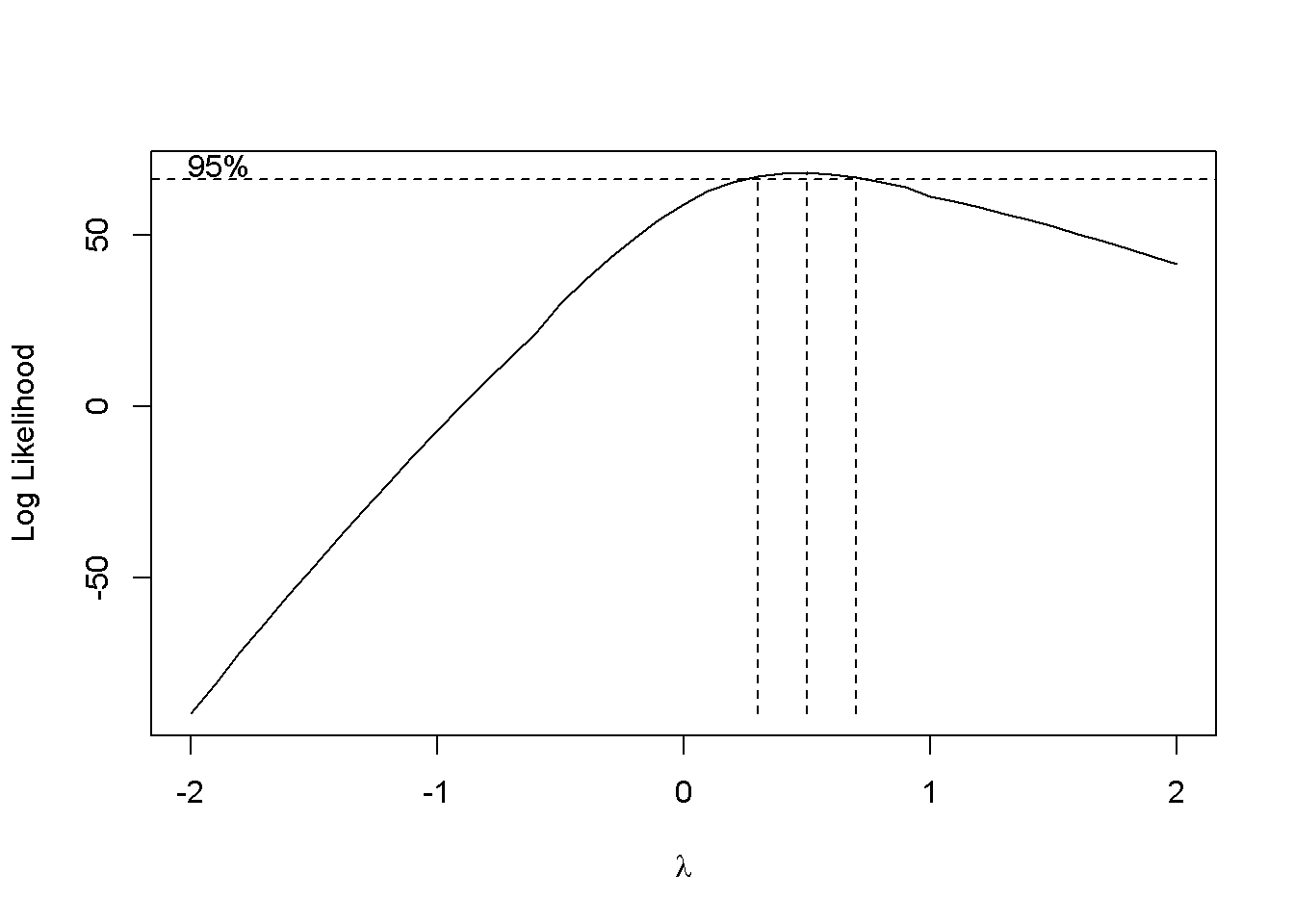
## [1] 0.3 0.7df <- read_csv(here::here("../imp_rmd/data/xiaosong-log-transformation.csv")) + 50.312312
df <-
df %>%
rename(score = score_v8_1)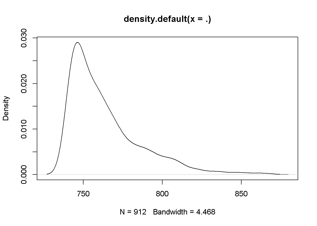
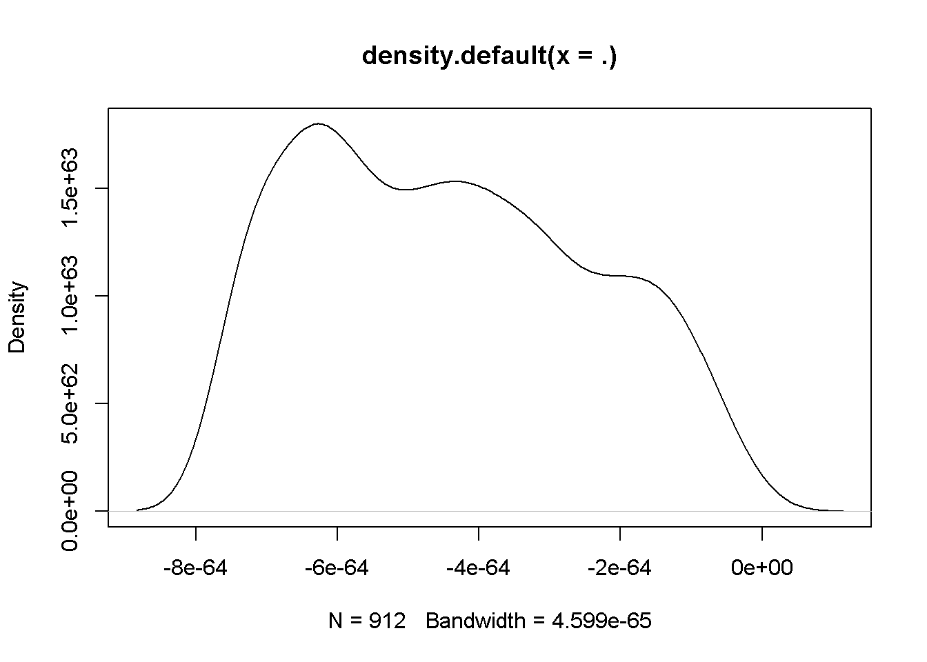
Figure 12.1: 通过转换后,分布趋近于正态分布了。
13 Power Transformation对预测能力的影响
Power Transformation 以下以变换作为简称。 假设回归方程为
\[y = \beta_0 + \beta_1 x + \mu\]
对\(y\)进行变化后,回归方程变成
\[\log(y) = \gamma_0 + \gamma_1 x + \nu\]
也许,
\[\text{p value}_{\hat \beta_1} > \text{p value}_{\hat \gamma_1}\]
因此经过变化后,回归系数的显著性上升。 但是,
\[R_{\hat \beta_1}^2 > R_{\hat \gamma_1}^2\]
回归方程的\(R^2\)可能会下降。
因为,
\[L = \frac{1}{2}\sum{(y-\hat y)^2} \to \frac{1}{2}\sum{(\log(y)-\widehat{\log(y)})^2}\]
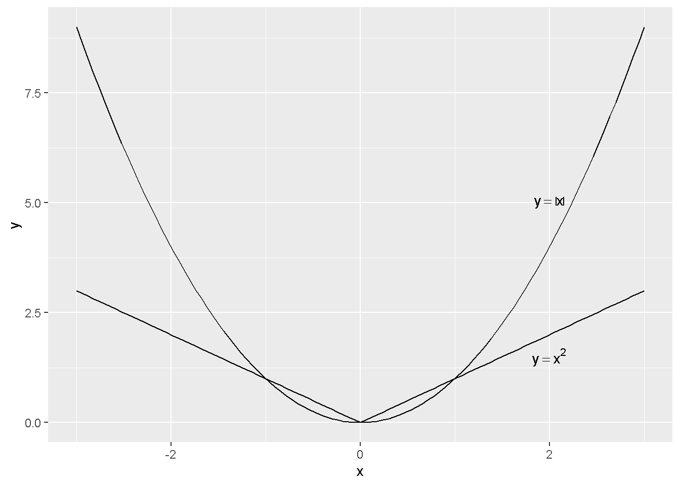
\(\log\)函数会将\(y\)的
- 较大值缩小更多
- 较小值缩小更少,
可以查看函数\(y = \log(x)\)的每个点的斜率来直观理解。
ggplot(data.frame(x = c(0.0001,100)), aes(x=x)) +
    stat_function(fun = function(x){log(x)}) +
    annotate("text", x=50, y=0, parse=TRUE, size=4,
             label="'Function: ' * y==log(x)")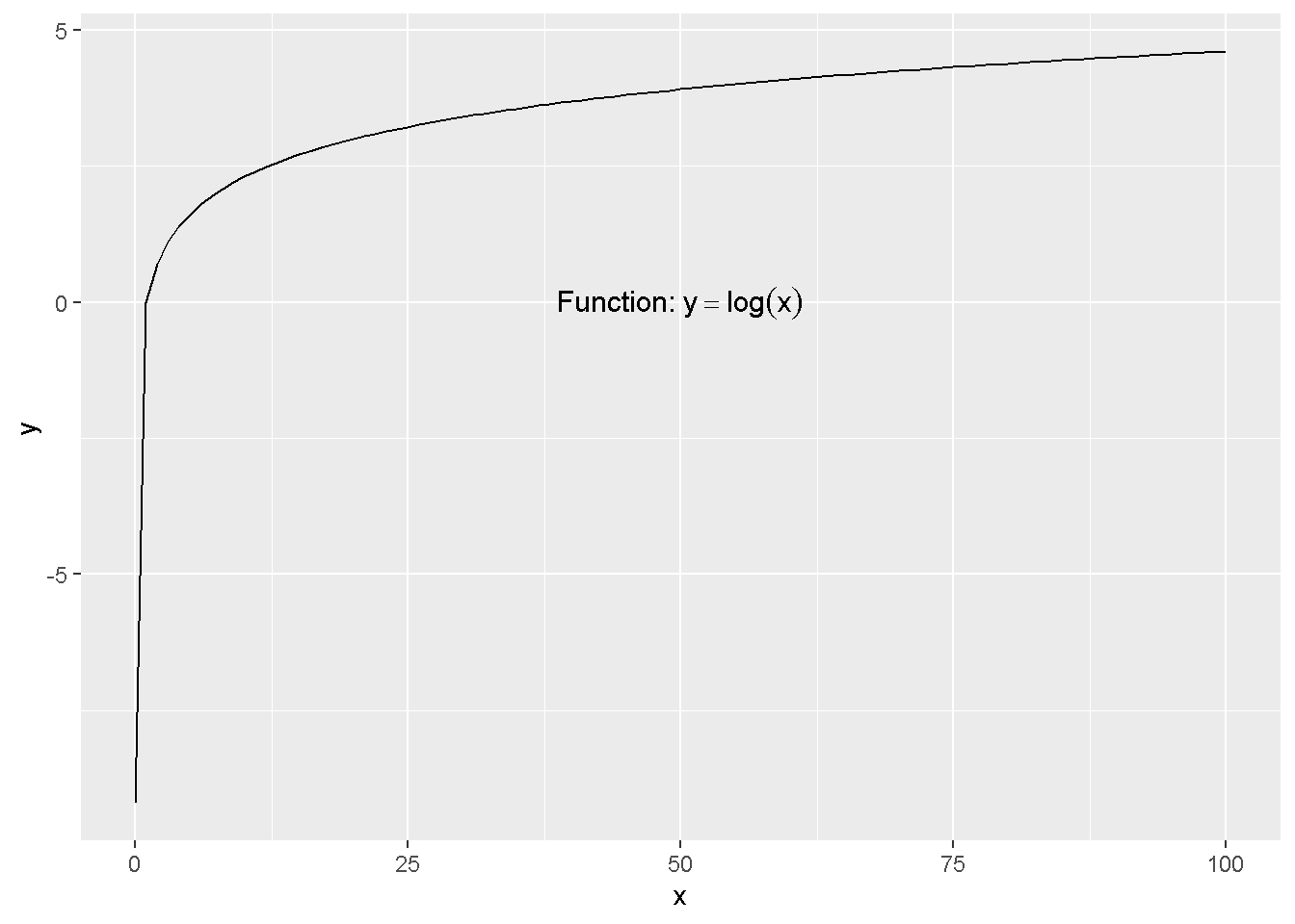
因此会对
- 较大值比较大的误差\(y-\hat y\)容易产生较小\(\log(y)-\widehat{\log(y)}\)
- 较小值比较小的误差\(y-\hat y\)容易产生较大\(\log(y)-\widehat{\log(y)}\)
这样一平均下来,
- 模型过分追求了较小值的误差纠正,因此较小值预测准确
- 放松了较大值的误差纠正,因此较大值预测非常不精确
这样一平均下来,
RMSE上升许多,模型效果下降。
14 Root Mean Squared Log Error RMSLE
Kaggle的比赛会使用到,如 House Prices 比赛,
Submissions are evaluated on Root-Mean-Squared-Error RMSE between the logarithm of the predicted value and the logarithm of the observed sales price. (Taking logs means that errors in predicting expensive houses and cheap houses will affect the result equally.)
RMSE 和 RMSLE 的区别就是对\(y\)和\(\hat y\)进行了对数处理,
\[y: \log(y+1)\]
因此,
\[\mathrm{RMSLE} = \sum(\log(y+1) - \log(\hat y + 1))^2\]
15 Generalized linear model GLM 模型
Yee (2015) 定义,
\[g(E(Y|X)) = \beta_1 x_1 + \cdots + \beta_p x_p\]
- \(E(Y|X)\)是一个均值函数
- \(g\)是一个抽象函数,可以是指数函数
这里是一个均值概念,是各个\(x\)与\(Y\)均值之间的关系,预测出来的\(\hat y\)也是估计\(E(Y|X)\)的。 这里跟OLS回归作区别。
16 指数回归
根据 15 公式,当
\[g = \log\]
公式简化为
\[E(y|x_1,x_2) = \exp(\beta_0 + \beta_1 x_1 + \beta_2 x_2) = \hat y\]
这是指数回归方程,也是指数关系的伽马回归方程 (Masterov 2014),详见 22。
这种回归区别于OLS,有三种解读。
16.1 marginal effects
\[\frac{\partial E(y|x_1,x_2)}{\partial x_1} = \exp(\beta_0 + \beta_1 x_1 + \beta_2 x_2) \cdot \beta_1 = \hat y \times \beta_1\]
因此\(x_1\)和\(\hat y\)之间的相关性,也受到\(\hat y\)的规模影响。
16.2 \(x_1\)是分类变量
\[\begin{alignat}{2} E(y|x_2, x_1 = 1) - E(y|x_2, x_1 = 0) &= (\exp(\beta_0 + \beta_1 + \beta_2 x_2)) - (\exp(\beta_0 + \beta_2 x_2)) \\ &= \exp(\beta_0 + \beta_2 x_2))(\exp(\beta_1) - 1) \\ \end{alignat}\]
\(x_1\)变动带来的影响,不仅仅是\(\beta_1\)。
16.3 \(x_1\)是连续变量
\[\begin{alignat}{2} E(y|x_2, x_1 + 1) &= \exp(\beta_0 + \beta_1 x_1 + \beta_1 + \beta_2 x_2) \\ &= \exp(\beta_0 + \beta_1 + \beta_2 x_2) \cdot \exp(\beta_1) \\ E(y|x_2, x_1) \cdot \exp(\beta_1) \\ \end{alignat}\]
\(x_1\)变动一个单位,\(\hat y\)是倍数变化而非加法变化。
17 onehot的bug
做one-hot虽然解决了部分无序类别的分类变量的排序问题, 但是这也导致了共线性发生的概率,
- 模型特征变量上升,共线性发生概率上升,
- 虽然两两之间的相关性在one-hot后下降,但是多变量之间的共线性上升了3。
18 无序类别变量进模型的处理方法
无序类别变量,例如省份,
- 可以进行one-hot编码,但是产生共线性等问题,详见 17
- 可以factor化,作为有序变量。排序逻辑,可以将身份 categorized化,然后对人均GDP,进行回归,取用\(\beta\)作为打分,或者再加入其他控制变量。 这时候有序变量就是单调的了,和WOE切分和树模型切分保持变量单调的思想一致的。
19 逻辑回归中,\(\beta\)的直观理解
\[\log(\frac{p}{1-p}) = \beta_0 + \beta_1 x + \mu\]
我们可以得到
\[\frac{p}{1-p} ~ \exp(\beta_1)\]
当\(x\)变动一个单位时,odd’s ratio增加\(\exp(\beta_1)\)个单位。
相关内容可以参考 Stack Exchange。
19.1 逻辑回归\(\hat z\)和\(\hat y\)切分使用条件
mtcars_sum <-
mtcars %>%
    select(vs,mpg,disp) %>%
    mutate(yhat = predict(mtcars_mod,type = 'response')) %>%
    mutate(zhat = predict(mtcars_mod)) %>%
    mutate(on = 1) %>%
    full_join(
        mtcars_mod %>%
            tidy() %>%
            select(1:2) %>%
            as.data.frame() %>%
            column_to_rownames(var = 'term') %>%
            t() %>%
            as.data.frame() %>%
            mutate(on = 1)
        ,by = 'on'
        ,suffix = c('_value','_beta')
    ) %>%
    mutate(z = `(Intercept)`+mpg_beta*mpg_value+disp_beta*disp_value
           ,y_hat_checked = 1/(1+exp(-z))

)##
## Welch Two Sample t-test
##
## data: mtcars_sum$yhat and mtcars_sum$y_hat_checked
## t = 5.8874e-16, df = 62, p-value = 1
## alternative hypothesis: true difference in means is not equal to 0
## 95 percent confidence interval:
## -0.18848 0.18848
## sample estimates:
## mean of x mean of y
## 0.4375 0.4375##
## Welch Two Sample t-test
##
## data: mtcars_sum$zhat and mtcars_sum$z
## t = 0, df = 62, p-value = 1
## alternative hypothesis: true difference in means is not equal to 0
## 95 percent confidence interval:
## -1.352149 1.352149
## sample estimates:
## mean of x mean of y
## -0.6703579 -0.6703579公式验证是无误的。 但是这里使用了
- \(\exp()\)和
- \(\frac{1}{1+()}\)
转置后,排序还是不发生改变,已经等样本给的切点是不会产生影响的。 因此,用\(\hat z\)切,和用\(\hat y\)切都一样。
20 树模型的距离问题
假设一个特征向量\(x\),有三个类别,\(\text{[red,blue,green]}\),作为一个string变量,强制factor化后,会标注为\(\text{[1,2,3]}\)。这种处理方法会使得出现red<blue<green,因为1<2<3,从而判断为错误的特征工程。
但是实际上是不用担心这个问题的(Zherebetskyy 2017)。
因此根据以上的信息增益的求解的讨论,树模型结构计算不是通过距离而计算的,而是找到信息增益最大的切分点(Jamshidi 2018)。在寻找最佳切分点时,这里只会产生两刀,1和2之间,或者2和3之间,尽量区分开\(y\),
因此split对red<blue<green这种排序时不敏感,因此不需要(但不是不能)进行OneHot处理。
综上,OneHot处理理论上优势不明显,而且还带来了缺点。 OneHot处理后自由度会下降。
21 泊松分布 (Poisson Distributions) 的推导
参考 李家伟 (2017) 和 Rodríguez (2007) 的推导过程。 从组合问题出发,柏松过程是一个二项分布问题。
这也是为什么柏松分布假设,样本间独立,因为二项分布就是样本独立的。
举个例子。
在一个无限空间口袋里,有无限多的黑球和白球,40%是黑球,60%是白球。分别拿三次球并记录每次拿出球的颜色,其中1个是白球,剩下2个是黑球的概率 P 是多少?
一般地,
在一个无限空间口袋里,有无限多的黑球和白球,\(p\)是黑球,\(1-p\)是白球。分别拿\(n\)次球并记录每次拿出球的颜色,其中\(k\)个是白球,剩下\(n-k\)个是黑球的概率\(P\)是多少?
这里相邻间的抽样是互不干扰的,因此相互独立。
解释完毕。
上述不考虑顺序的话,概率为
\[P = p^k(1-p)^{n-k}\]
上述考虑顺序的话,概率为
\[P = C_{n}^kp^k(1-p)^{n-k} = \frac{\frac{n!}{(n-k)!}}{k!}c=\frac{n!}{(n-k)!k!} \cdot p^k(1-p)^{n-k}\]
这个是推导基础。
假设单位时间内,平均抽取的黑球数量为\(\lambda = np\)。 因为假设单位时间为一年,一次实验进行1个月,那么一年有12次,每次概率为\(p\),因此黑球的期望是\(\hat \lambda = 12 \cdot p\),这里的\(\hat n = 12\),因此\(\lambda = np\)。
因此,
\[\begin{alignat}{2} P & = \frac{n!}{(n-k)!k!} \cdot p^k(1-p)^{n-k} \\ & = \frac{n!}{(n-k)!k!} \cdot {(\frac{\lambda}{n})}^k(1-\frac{\lambda}{n})^{n-k} \\ & = \frac{n!}{(n-k)!k!} \cdot {(\frac{\lambda}{n})}^k \cdot \frac{(1-\frac{\lambda}{n})^{n}}{(1-\frac{\lambda}{n})^{k}}\\ & = \frac{n!}{(n-k)!n^k}\cdot \frac{1}{k!} \cdot \lambda^k \cdot \frac{(1-\frac{\lambda}{n})^{n}}{(1-\frac{\lambda}{n})^{k}}\\ \end{alignat}\]
其中,
\[\begin{alignat}{2} \frac{n!}{(n-k)!n^k} & = \frac{n(n-1)(n-2)\cdots(n-k+1)}{n^k} \\ & = (1)(1-\frac{1}{n})(1-\frac{2}{n})\cdots(1-\frac{k-1}{n}) \\ & \to 1 \end{alignat}\]
如果\(p =\frac{\lambda}{n}\)很小,\(1-p \to 1\)
所以,
\[(1-\frac{\lambda}{n})^k \to 1^k = 1\]
最后,
\[(1-\frac{\lambda}{n})^n = (1+\frac{1}{\frac{n}{-\lambda}})^{\frac{n}{-\lambda} \cdot -\lambda} = e^{-\lambda}\]
所以,
\[P = \frac{1}{k!}\lambda^ke^{-\lambda}\]
下一步是如何理解泊松分布的回归方程。
\[\log(\lambda) = X \times \beta\]
这里理解,\(\lambda = np\)是单位时间内的期望数量。 \(P\)是当单位时间内的期望数量为\(\lambda\),产生\(k\)次黑球的概率。
22 Gamma 回归方程
gamma回归方程是相当于因变量\(y\)符合gamma分布而言的。 gamma回归方程属于GLM的一种,详见 15,因此\(\hat y\)也是针对\(E(Y|X)\)而言,这里和OLS回归区别。
22.1 Gamma 分布 (Li 2018a)
\[Y \sim \Gamma(\alpha, \beta)\]
有两个性质
\[\begin{cases} E(y_i) = \alpha_i \cdot \beta_i \\ Var(y_i) = \alpha_i \cdot \beta_i^2 \\ \end{cases} \to \frac{Var(y_i)}{E(y_i)} = \beta_i\]
因此和 log变换的假设不一致,见 22.5。
22.2 Gamma 回归方程的作用
当我们发现\(y\)变量符合一些特征,当均值增加(减少)时,方差也随着增加(减少),我们可以认为\(y\)可能符合 Gamma 分布。(Johnson 2014, Section 6) 例如,房价,在低位时波动少,高位时波动大。
22.3 和lognormal分布的相同点
Stack Exchange (2013b) 认为, Gamma分布和log transformation的处理,会依据数据来操作,但数据基本是上符合这样的特征:
- 连续的
- 非负的
- 右偏的
但是处理的程度不同。

- 左上和右上两图分别用lognormal和gamma分布模拟出来,
- 中一和中二都使用lognormal进行变换,发现只有左图比较符合正态分布,右图处理过渡,产生了左偏。
- 左下和右下都使用了cuberroot进行变换,发现只有有图比较符合正态分布,左图处理不够,还有右偏。 (Stack Exchange 2013a)
22.4 和OLS回归的不同
当我们发现\(y\)变量符合一些特征,当均值增加(减少)时,方差也随着增加(减少),另外一种处理方式是进行Power Transformation,简单的做法是\(\log\)处理,详见 13的讨论,这并不有效。 房价比赛 的预测发现,\(\log\)处理后的预测能力下降。 但这并不是说OLS回归比Gamma回归差,哪一个有效,更多的说明,因变量更符合哪个分布。
这里的本质区别是,
- 指数回归,作为一种特殊的Gamma回归,是对\(E(Y|X)\)进行处理,形成\(\log(E(Y|X))\)
- OLS回归,是对\(Y\)进行处理,形成\(E(\log(Y|X)\) (Johnson 2014, Section 3)
\[\log(E(Y|X)) \neq E(\log(Y|X)\]
我几次项目和比赛的经验是,OLS回归中的\(Y\)进行Power Transformation,效果都不理想。
22.5 log变换的推导
- log变换假设均值和标准差成正比 (姚岑卓 2017; Li 2018a)
- gamma分布假设均值和方差成正比
假设一个时间序列的例子,标准差伴随均值增加(房价具备这样的特性)。
\[\sqrt{\mathrm{Var}(X_t} = \mathrm{E}(X_t) \sigma\]
那么,
\[\begin{alignat}{2} X_t &= X_t\\ & = \mathrm{E}(X_t) \cdot \frac{X_t}{\mathrm{E}(X_t)} \\ & = \mathrm{E}(X_t) \cdot \frac{X_t - \mathrm{E}(X_t) + \mathrm{E}(X_t)}{\mathrm{E}(X_t)} \\ & = \mathrm{E}(X_t) \cdot (1 + \frac{X_t - \mathrm{E}(X_t)}{\mathrm{E}(X_t)}) \\ \end{alignat}\]
利用log函数的处理4,
\[\log(1+x) \approx x\] \[\log(1 + \frac{X_t - \mathrm{E}(X_t)}{\mathrm{E}(X_t)}) = \frac{X_t - \mathrm{E}(X_t)}{\mathrm{E}(X_t)}\]
所以,
\[\begin{alignat}{2} X_t &= \mathrm{E}(X_t) \cdot (1 + \frac{X_t - \mathrm{E}(X_t)}{\mathrm{E}(X_t)}) \\ \log X_t &= \log \mathrm{E}(X_t) + \log (1 + \frac{X_t - \mathrm{E}(X_t)}{\mathrm{E}(X_t)}) \\ &= \log \mathrm{E}(X_t) + \frac{X_t - \mathrm{E}(X_t)}{\mathrm{E}(X_t)} \\ \mathrm{E}(\log X_t) & \approx \log \mathrm{E}(X_t) \end{alignat}\]
22.6 gamma回归在实际操作的优势
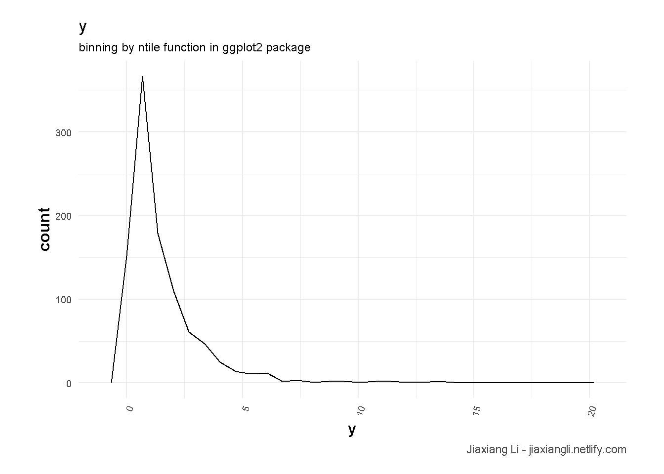
set.seed(1111)
n <- 1000
df <- tibble(
y = rnorm(n, mean=0, sd=1) %>% exp()
) %>%
mutate(
x = log(y) - rnorm(n, mean=0, sd=1)
)
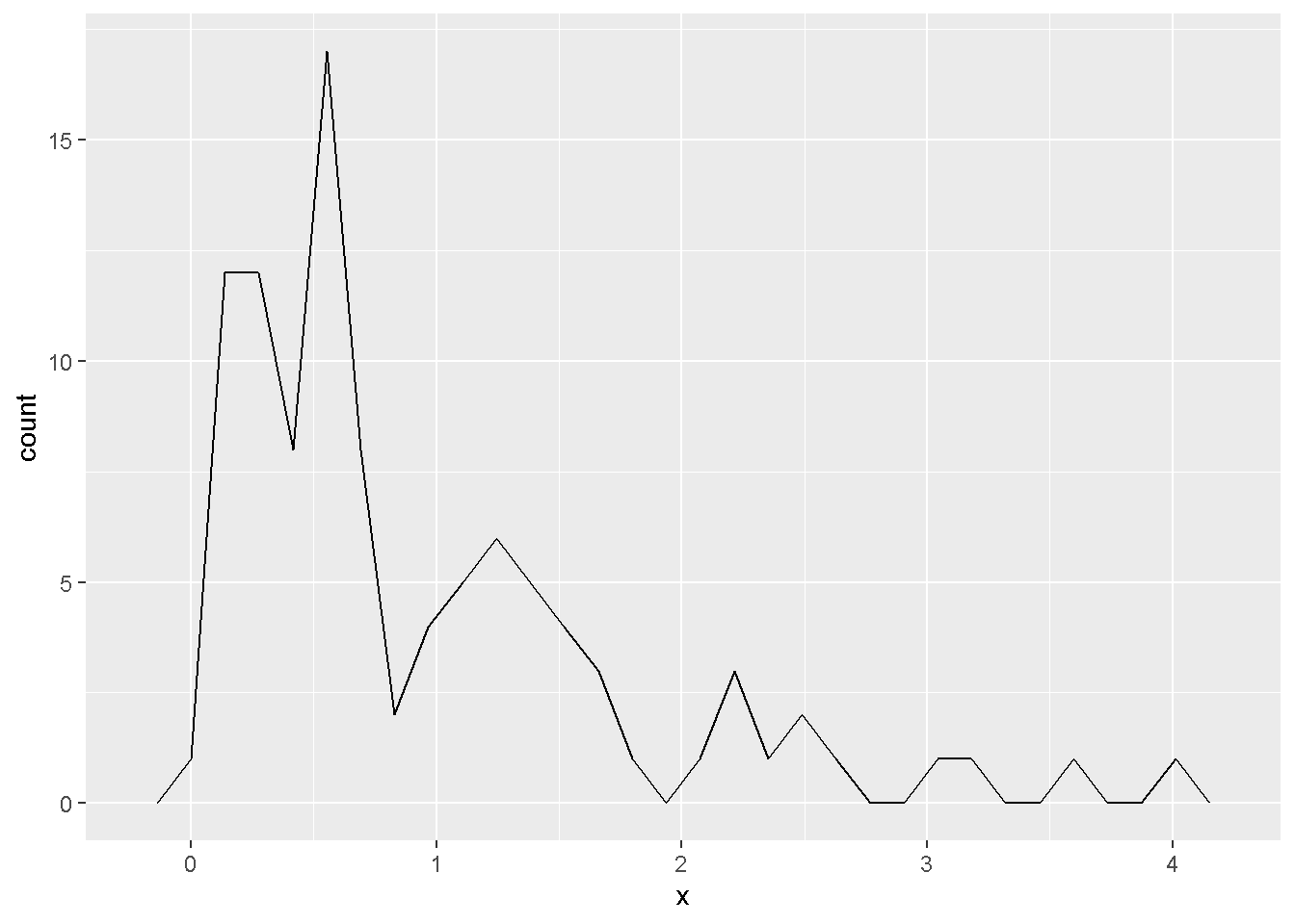
dfdf %>%
ggplot(aes(x = y)) +
geom_freqpoly() +
theme_ilo() +
labs(
title = "y",
subtitle = "binning by ntile function in ggplot2 package",
caption = "Jiaxiang Li - jiaxiangli.netlify.com"
)
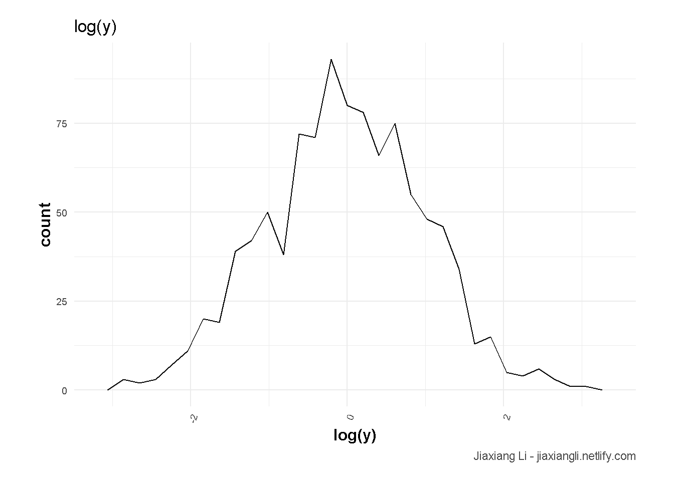
df %>%
    ggplot(aes(x = log(y))) +
    geom_freqpoly() +
    theme_ilo() +
    labs(
        title = "log(y)",
        caption = "Jiaxiang Li - jiaxiangli.netlify.com"
    )
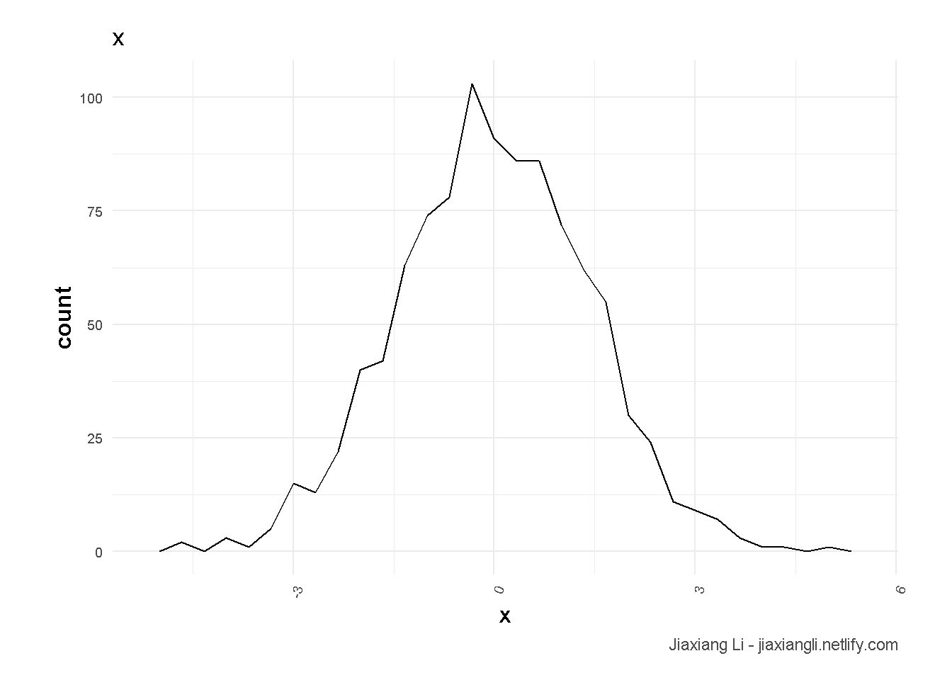
df %>%
    ggplot(aes(x = x)) +
    geom_freqpoly() +
    theme_ilo() +
    labs(
        title = "x",
        caption = "Jiaxiang Li - jiaxiangli.netlify.com"
    )
例子来自 Stack Exchange (2012a)。
y <- rnorm(n, mean=0, sd=1)
y <- exp(y)- 说明\(y\)一个lognormal类型的变量。
- 明显的右偏。
lm <- lm(y ~ x, data = df)
log_lm <- lm(log(y) ~ x, data = df)
log_gauss_glm <- glm(y ~ x, data = df, family=gaussian(link="log"))
log_gamma_glm <- glm(y ~ x, data = df, family=Gamma(link="log"))library(formattable)
df_add_pred <-
df %>%
mutate(
lm_pred = predict(lm),
log_lm_pred = predict(log_lm) %>% exp(),
log_gauss_glm_pred = predict(log_gauss_glm, type="response"),
log_gamma_glm_pred = predict(log_gamma_glm, type="response"),
) %>%
gather(key,value, lm_pred:log_gamma_glm_pred)
df_add_pred %>%
ggplot() +
geom_point(aes(x = x, y = y)) +
geom_line(aes(x = x, y = value, col = key))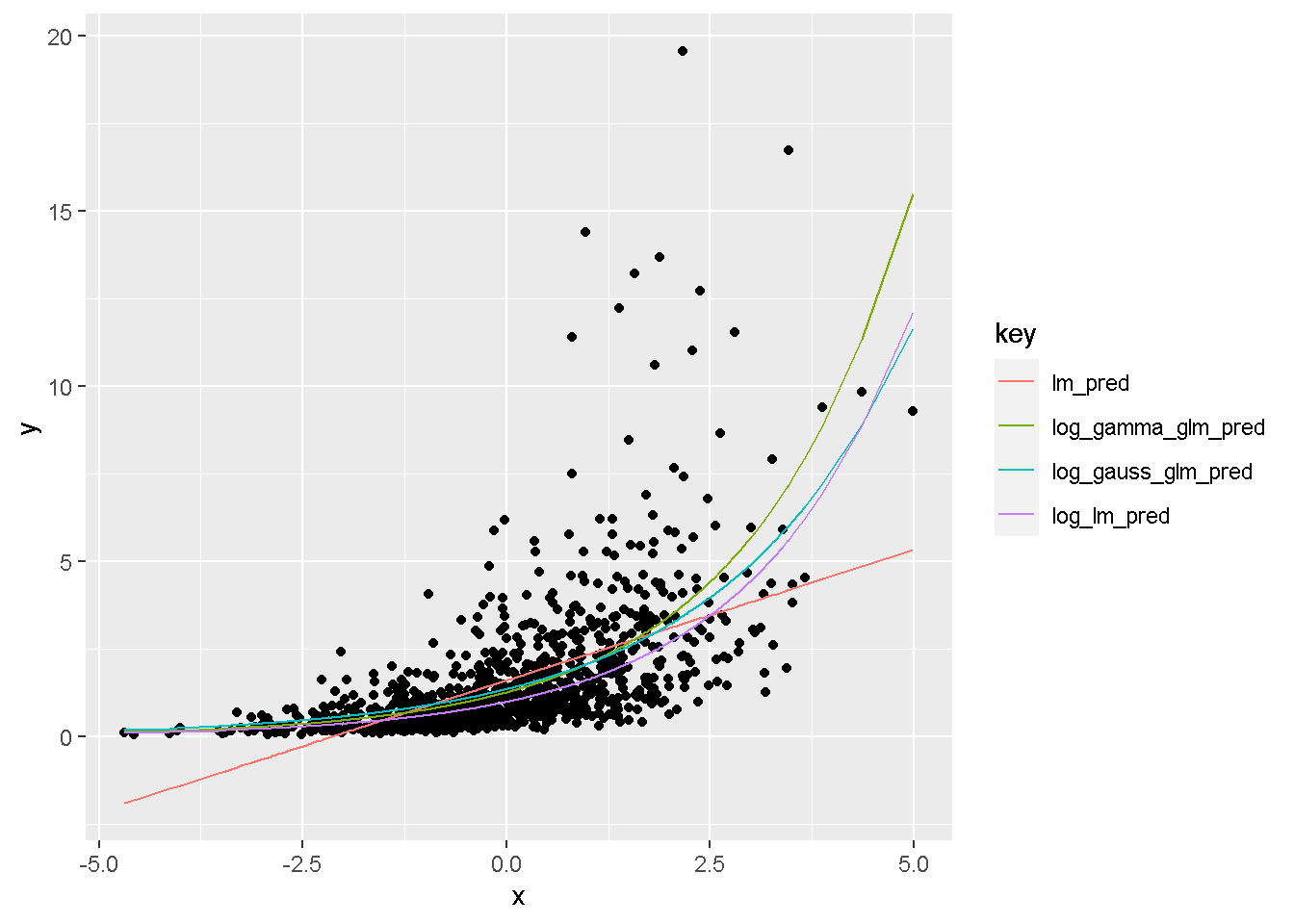
- 我们发现除了
lm_pred,其他拟合线都是弯的。 log_lm_pred和log_gamma_glm拟合最好,即使\(y\)变量是lognormal分布的,而非gamma分布,log_gamma_glm依然表现很好。
23 tweedie 回归
tweedie 回归表达了 \(\mathrm{Var}(y) \sim \mathrm{E}(y)^\text{tweedie variance power}\)(DMLC 2018)。
因此,显然比 Gamma 回归 (见 22) 更加的宽泛,因此假设上更加的普遍使用。 在Xgboost中,tweedie variance power 的默认值为1.5(DMLC 2018),因此为了进行模型的更优化测试,我建议可以一开始就先进行 tweedie variance power 的调整参数。
\[\text{tweedie variance power} \in (1,2)\]
- 越接近2,越拟合成Gamma回归
- 越接近1,越拟合成Possion回归
Tweedie 回归、Gamma 回归 (见 22) 主要应用于有右偏的数据,如保险等。 更多可以查看Github上的这篇 讨论。
24 Tweedie tuning power
进行回归时,可以先研究y变量的分布。 同样可以使用QQ图进行研究,见 5 Q-Q 图理解 。 特别地,当分布满足tweedie需要进行对power进行估计。 比如,Xgboost中,需要对其进行研究。 研究的思路主要参考 jlhoward (2017) 。
library(tweedie)
library(data.table)
tweedie_data <-
    rtweedie(
        n = 100
        ,power= 2.5
        ,mu = 1
        ,phi = 1
    ) %>%
data.table(x=.)- 我们sim一个数据,
power=2.5
- 符合Gamma分布类的数据,右偏倾向。
params <- list(
    power= 2.5
    ,mu = 1
    ,phi = 1
)
library(tweedie)
tweedie_data %>%
    ggplot(aes(sample=x)) +
    stat_qq(distribution=tweedie::qtweedie,dparams=params) +
    stat_qq_line(distribution=tweedie::qtweedie,dparams=params)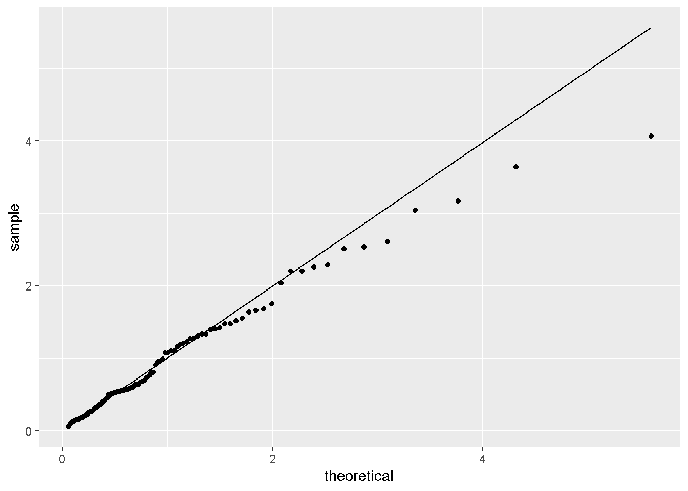
- QQ图符合。
params <- list(
    power= 2.0
    ,mu = 1
    ,phi = 1
)
tweedie_data %>%
    ggplot(aes(sample=x)) +
    stat_qq(distribution=tweedie::qtweedie,dparams=params) +
    stat_qq_line(distribution=tweedie::qtweedie,dparams=params)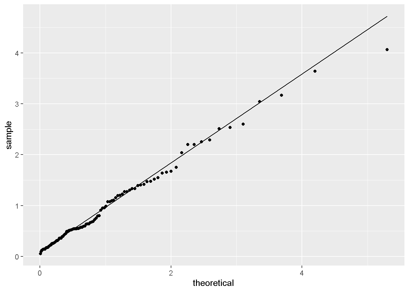
- QQ图不符合。
params <- list(
    power= 1.5
    ,mu = 1
    ,phi = 1
)
library(tweedie)
tweedie_data %>%
    ggplot(aes(sample=x)) +
    stat_qq(distribution=tweedie::qtweedie,dparams=params) +
    stat_qq_line(distribution=tweedie::qtweedie,dparams=params)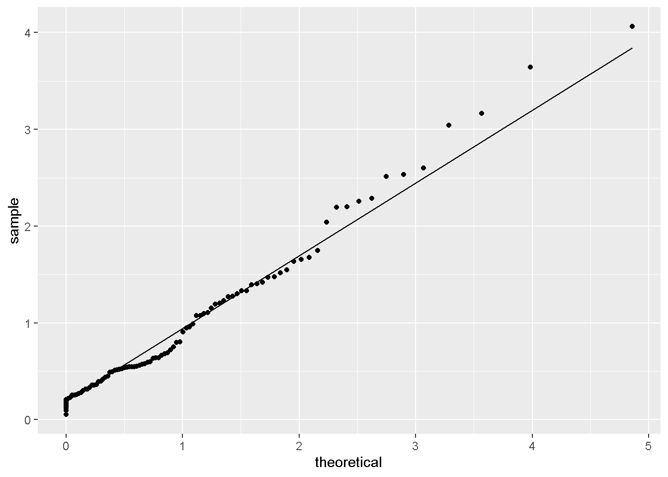
- QQ图不符合。
params <- list(
    power= 1.0
    ,mu = 1
    ,phi = 1
)
library(tweedie)
tweedie_data %>%
    ggplot(aes(sample=x)) +
    stat_qq(distribution=tweedie::qtweedie,dparams=params) +
    stat_qq_line(distribution=tweedie::qtweedie,dparams=params)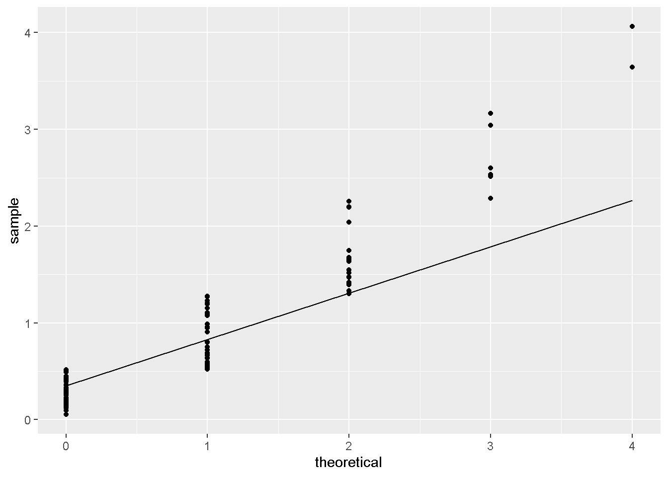
- QQ图不符合。
- run起来比较慢。
DiFranco (2016) 给出了限定tweedie_variance_power的方式,可以参考。
同时,
Stack Overflow上也有相应的讨论。
params <- list(
  objective = 'reg:tweedie',
  eval_metric = 'rmse',
  tweedie_variance_power = 1.4,
  max_depth = 6,
  eta = 1)

bst <- xgb.train(
  data = d_train,
  params = params,
  maximize = FALSE,
  watchlist = list(train = d_train),
  nrounds = 20)
25 Install lightgbm for python 2 on Win 7 and Mac (Python Software Foundation 2018)
pip install lightgbm如果报错
grin 1.2.1 requires argparse>=1.1, which is not installed.执行 见csdn
pip install argparse26 logit vs. probit model
probit模型是基于累计正态分布而言的。 分别对比 probit 和 logit的和分布和一阶偏导分布,会发现 probit 在尾部更平(Stack Exchange 2012b; Sanchez 2017)。 因此可以确定probit 预测的概率\(\in [0,1]\)。


26.0.1 公式证明 (Lee 2014; Wikipedia contributors 2018a)
\[\mathrm{Pr}(Y = 1 | X) = \Phi(X^T\beta)\]
假设
\[Y^* = X^T \beta + \varepsilon\]
这里\(\varepsilon\)满足
\[\varepsilon \sim N(0,1)\]
因此,有
\[Y = \begin{cases} 1 & Y^* > 0 \\ 0 & \mathrm{otherwise} \\ \end{cases} = \begin{cases} 1 & - \varepsilon < X^T \beta \\ 0 & \mathrm{otherwise} \\ \end{cases}\]
这里\(Y\)和\(- \varepsilon < X^T \beta\)的联系在,
\[\begin{alignat}{2} \mathrm{Pr}(Y=1|X) &= \mathrm{Pr}(Y^* > 0) \\ &= \mathrm{Pr}(X^T \beta + \varepsilon > 0) \\ &= \mathrm{Pr}(\varepsilon > - X^T \beta) \\ &\xrightarrow{正态分布对称性} \mathrm{Pr}(\varepsilon < X^T \beta) \\ &= \Phi (X^T \beta) \end{alignat}\]
26.0.2 最大似然估计
logit 和 线性SVM用到,
\[\begin{alignat}{2} \text{Cost} & = -[\overbrace{y\log (h_{\theta}(x))}^{\text{y = 1}}+\overbrace{(1-y)\log(1-h_{\theta}(x))}^{\text{y = 0}}] \\ & = -y\log\frac{1}{1+e^{-\theta^Tx}}-(1-y)\log(1-\frac{1}{1+e^{-\theta^Tx}}) \end{alignat}\]5
probit (Lee 2014, 177–180;@wikiProbit)用到,
\[\begin{alignat}{2} L & = \prod_{i=1}^N \overbrace{\Phi(X^T\beta)^y}^{\text{y = 1}} \cdot \overbrace{(1-\Phi(X^T\beta)^{1-y}}^{\text{y = 0}} \\ \end{alignat}\]
\[\begin{alignat}{2} \log(L) & = \sum_{i=1}^N \overbrace{y \log (\Phi(X^T\beta))}^{\text{y = 1}} + \overbrace{(1-y) \log (1-\Phi(X^T\beta)}^{\text{y = 0}} \\ \end{alignat}\]
比较类似。
26.0.3 \(y\)的倍数
Lee (2014, 180) 给出了经验性法则,
\[y_{\mathrm{logit}}^* = 1.8 \cdot y_{\mathrm{probit}}^*\]
注意这里
\[y \neq y^* = X^T \beta + \varepsilon\]
因为,
- logit的均值为0,方差为\(\frac{\pi^2}{3}\)
- probit的均值为0,方差为1的正态分布
因此,倍数为\(\frac{\pi}{\sqrt{3}} = 1.8128798\)
27 房价取log变换的依据
假设房的需求和人口成正比,
不考虑其他因素的情况下,生物的种群总是指数增长的 (慧航 2014),
\[\frac{dP}{dt} = rP\]
\(P\)表示人口,\(r\)表示自然增长率。
当做log变换时,
\[\frac{d \log P}{dt} = \frac{d \log P}{dp} \cdot \frac{d P}{dt} = \frac{1}{P} \cdot rP = r\]
问题就更加简单的研究了。
28 MAE 和 MSE 的比较
- MAE: L1 损失
- MSE: L2 损失
文本参考 Shukla (2015) 和 张建军 (2018) 。
28.1 对异常值的敏感程度
MAE_MSE_comp <-
tibble(
    Err = c(0,1,-2,-.5,1.5)
) %>%
    mutate(AE = abs(Err-mean(Err)),
           SE = (Err-mean(Err))^2)
MAE_MSE_comp
MAE_MSE_comp_sum <-
MAE_MSE_comp %>%
summarise(MAE = mean(AE),
MSE = sqrt(mean(SE))) %>%
mutate_all(accounting)
MAE_MSE_comp_sumMAE_MSE_comp2 <-
tibble(
Err = c(0,1,1,-2,150)
) %>%
mutate(AE = abs(Err-mean(Err)),
SE = (Err-mean(Err))^2)
MAE_MSE_comp2MAE_MSE_comp_sum2 <-
MAE_MSE_comp2 %>%
summarise(MAE = mean(AE),
MSE = sqrt(mean(SE))) %>%
mutate_all(accounting)
MAE_MSE_comp_sum2MAE_MSE_comp_sum %>% bind_cols(MAE_MSE_comp_sum2) %>%
transmute(MAE_ratio = MAE1/MAE,
MSE_ratio = MSE1/MSE)AE和SE分别表示 Ave. Error 和 Squared Error。
看以上例子可以发现,当训练集中,有异常值时,
MAE误差增加的幅度没有MSE高。因此当数据对离群点敏感时,建议用MAE。
29 ARIMA模型加入多个x变量
Raad (2015) 给予了auto.arima函数中多个\(x\)变量的情况,并且forecast函数执行成功,以下是小例子,实验数据下载见 这里。
dta <- read.csv("xdata.csv")[1:96,]
dta <- ts(dta, start = 1)

# to illustrate out of sample forecasting with covariates lets split the data
train <- window(dta, end = 90)
test <- window(dta, start = 91)

# fit model
covariates <- c("DayOfWeek", "Customers", "Open", "Promo", "SchoolHoliday")
fit <- auto.arima(train[,"Sales"], xreg = train[, covariates])

# forecast
fcast <- forecast(fit, xreg = test[, covariates])
30 在R中使用逻辑回归
help(family): Family Objects for Models- 主要常用函数参考 Kabacoff (2017)
# Logistic Regression
# where F is a binary factor and
# x1-x3 are continuous predictors
fit <- glm(F~x1+x2+x3,data=mydata,family=binomial())
summary(fit) # display results
confint(fit) # 95% CI for the coefficients
exp(coef(fit)) # exponentiated coefficients
exp(confint(fit)) # 95% CI for exponentiated coefficients
predict(fit, type="response") # predicted values
residuals(fit, type="deviance") # residuals
predict(fit, type="response")和residuals(fit, type="deviance")可以帮助手动版本的集成算法。
31 rfm模型介绍
RFM是三种客户行为的英文缩写(杜雨 2018)。
- Recency (t) How recently did the customer purchase?
- 体现用户留存
- 客户最近一次交易时间的间隔。R值越大,表示客户交易距今越久,反之则越近;
- Frequency (n) How often do they purchase?
- 体现用户活跃度
- 客户在最近一段时间内交易的次数。F值越大,表示客户交易越频繁,反之则不够活跃;
- Monetary Value ($) How much do they spend?
- 体现用户价值。
- 客户在最近一段时间内交易的金额。M值越大,表示客户价值越高,反之则越低。
用户评级权重依次为,R > F > M。 分别与时间、次数、金额有关,用来衡量客户的价值。 注意每个变量并非单调。
下面主要讲建模的思路。 建模的思路和数据参考 Lantz (2017 Chapter 3)。
这里进行数据介绍。
donors数据
,下载地址这里
,含有93,462个瘫痪的残疾军人样本,通过信封沟通得到的数据。
其中变量解释如下
donated: 是否会捐款,1会,0不会,这讲作为逻辑回归的因变量。bad_address: 邮箱地址比较差,1是,0不是,可以认为降低捐款的概率interest_religion: 宗教interest_veterans: 对老兵的兴趣,增加捐款的概率
donors <- read_csv("https://assets.datacamp.com/production/course_2906/datasets/donors.csv")

# Build a recency, frequency, and money (RFM) model
rfm_model <- glm(donated ~ recency * frequency * money, data = donors)

# Summarize the RFM model to see how the parameters were coded
rfm_model %>% tidy() %>% kable()

# Compute predicted probabilities for the RFM model
rfm_prob <- predict(rfm_model, type = "response")

# Plot the ROC curve and find AUC for the new model
library(pROC)
ROC <- roc(donors$donated, rfm_prob)
plot(ROC, col = "red")
auc(ROC)这是RFM的8种状态,对于三个变量进行交叉项目设置后,
recency * frequency * money,模型会产生7个变量和1对照组,由于分类变量的设置,每组之间都是互斥的,进而可以查看每个交叉项的显著水平和局部效应。
32 方差膨胀系数(VIF)
方差膨胀系数 ,又称Variance inflation factor ,简称VIF。定义参考 Wikipedia contributors (2018b)。
\[Y = \beta_0 + \beta_1 X_1 + \cdots + \beta_n X_n + \mu\]
对于这个方程,我们计算\(X_1\)的VIF,作
\[X_1 = \alpha_1 + \alpha_2 X_2 + \cdots + \alpha_n X_n + \nu, R_1^2\]
其中\(\hat \beta_1\)的VIF为
\[\text{VIF}_1 = \frac{1}{1-R_1^2}\]
同时存在
\[\begin{alignat}{2} \hat{\text{var}}(\hat beta_1) &= \frac{\text{RMSE}^2}{(n-1)\hat{\text{var}}(X_1)}\cdot \frac{1}{1-R_1^2} \\ &= \frac{\text{RMSE}^2}{(n-1)\hat{\text{var}}(X_1)}\cdot \text{VIF}_1 \\ \end{alignat}\]
因此,
当\(X_1\)和其他变量不线性相关时,定义为best的情况,
\[R_1^2 = 0 \to (\text{VIF}_1^{\text{best}} = \frac{1}{1-0}) = 1\]
\[\frac{\hat{\text{var}}(\hat beta_1)}{\hat{\text{var}}(\hat beta_1)^{\text{best}}} = \frac{\text{VIF}_1}{1}\]
当\(\text{VIF}_1=m\)时,\(\hat{\text{var}}(\hat beta_1)\)比最好情况时,大\(\sqrt{m}\)倍,一般\(\sqrt{10}\),或者VIF=10是比较好的cutoff6。
R中可以使用,car::vif
> library(car)
> vif(spend.m2)
age credit.score email distance.to.store
1.094949 1.112784 1.046874 1.297978
online.visits online.trans store.trans store.spend
8.675817 8.747756 125.931383 123.435407
...
更多例子可以查看 Marketing Analytics in R: Statistical Modeling 学习笔记 。
33 需求、KPI的预测经验
对需求 (demand)、经营计划KPI定制、营收之类的预测,如果直接用时间序列或者大模型,容易过拟合,因为自由度不够,大多数是年度或者月度数据。 其次,回归、ARIMA是比较好的baseline模型,可以帮助先查看一下数据(LaBarr 2018; Warden 2018; 申利彬 and 丁楠雅 2018)。
对于样本小的问题,偏好使用计量的经典模型进行预测,然后做 集成 (blending) 或者层级预测 (Hierarchical forecasting) (LaBarr 2018)。
以下介绍主要的操作步骤。
33.1 集成
营收的预测可以用两个模型和两者的集成
\[\begin{cases}
\text{ARIMA} \\
\text{Regression} \\
\mathrm{LTSM \dots} \\
\text{Ensemble}
\begin{cases}
\text{ave.} \\
y \sim y_1 + y_2 \\
\end{cases}
\end{cases}
\xrightarrow{
[y \to \log y]\to[\hat{\log y}\to \exp(\hat{\log y})]\\
}
\text{Use Valid Set to choose best}\]
这个思想是博众家之长,观点也不是新颖,但是操作起来非常简单,
我参考了下 LaBarr (2018 Chapter 3),基本上使用R的auto.arima(跳过检验等繁琐步骤)和lm函数即可迅速完成,节省了神经网络、树模型超参数调整的时间。
最后一步选模型是值得启发的。LaBarr (2018 Chapter 3.9,3.13)似乎觉得集成并不一定好的事实普遍存在,因此不必纠结集成后效果一定好,LaBarr (2018 Chapter 3.9,3.13)经验地 认为大概率就是不好的,这里择优处理即可。
对于ARIMA 和 Regression 可以合并,相当于在ARIMA模型中加入x变量。但是时间上有些困难,因为auto.arima中的xreg参数负责加入x变量,操作容易出bug。加x参数还是lm最稳定。
33.2 层级预测
这里分为自下而上 (bottom-up)、自上而下 (top-down) 两种方式。(LaBarr 2018, Chapter 4) 对于比赛而言,只需要使用第一种。 对于KPI定制而言,第二种可以减少定制时间。
33.3 自下而上
\[\begin{cases} a_1 = f(\dots) \to \hat a_1\\ a_2 = f(\dots) \to \hat a_2\\ a_3 = f(\dots) \to \hat a_3\\ \end{cases} \xrightarrow{A = a_1 + a_2 + a_3} \hat A = \hat a_1 + \hat a_2 + \hat a_3\]
显然这里存在优点和值得讨论的缺点。
- 优点
- 训练速度快,
- 最后总误差是小于直接预测\(\hat A\)的
- 这种分步操作,符合实操中版本控制、上线计划、便于修改
- 缺点
- 分步操作其实也多使用了自由度,相当于增加了整体模型的参数,容易 过拟合。
- 但是样本小而过拟合是不可避免的,但是基于分步操作,过拟合易于修改、迭代,也就不是问题了。
33.4 MAPE
\[MAPE = \frac{1}{n}\sum\frac{\mathrm{y-\hat y}}{y}\](LaBarr 2018, Chapter 1.9)
34 random forest SQL上部署
library(randomForest)
library(tidypredict)
library(tidyverse)
set.seed(123)
diamonds_sub <-
    diamonds %>%
    sample_n(100)
model <-
    diamonds %>%
    randomForest(carat ~ ., data = ., ntree=3)
model %>%
    tidypredict_sql(dbplyr::simulate_mssql()) %>%
    write_file('tmp_rf_logic.sql')
diamonds_sub %>%
mutate(pred = case_when(...)) %>%
select(cut,pred) %>%
group_by(cut,pred) %>%
count() %>%
spread(pred,n)tidypredict_sql(model, dbplyr::simulate_mssql())可以给SQl 的CASE WHEN的规则,作为策略,方便交流。tidypredict_fit可以给dplyr 的case_when的规则,作为策略,方便交流。model %>% parse_model()给出了使用的变量、路径和路径方向,做出预测,然后算\(\hat y\)概率,作为切bin而用。
35 随机森林中加入MA和RSI因子
George (2018) 给出了预测股价的一个方法论,对于股价这种时间序列,
- 如果单纯作为横截面数据预测,效果不会理想
- 如果使用ARIMA模型,无法使用标准的树结构模型
因此考虑使用MA和RSI数据进入树结构模型,兼顾时间序列和树模型。
利用周期性,加入星期几数据,这种周期指标有两个好处,
- 未来一定存在,
- 具备周期性,因此效果不会太差。
MA数据,可以作用到200天,如果数据量足够的话。
RSI的指标定义为
\[RS = \frac{\text{Ave. Gain over n periods}}{\text{Ave. Loss over n periods}}\] \[RSI = 100 - \frac{100}{1+RS}\]
George (2018) 实现方式在Python,以下部分函数和技巧可以借鉴。
shift函数是lag和lead的替代。pct_change函数也有shift的作用。(George 2018,Chapter 1.2)
MA和RSI指标可以使用for循环完成。(George 2018,Chapter 1.5)
feature_names = ['5d_close_pct']  # a list of the feature names for later

# Create moving averages and rsi for timeperiods of 14, 30, 50, and 200
for n in [14,30,50,200]:

    # Create the moving average indicator and divide by Adj_Close
    lng_df['ma' + str(n)] = talib.SMA(lng_df['Adj_Close'].values,
                              timeperiod=n) / lng_df['Adj_Close']
    # Create the RSI indicator
    lng_df['rsi' + str(n)] = talib.RSI(lng_df['Adj_Close'].values, timeperiod=n)

    # Add rsi and moving average to the feature name list
    feature_names = feature_names + ['ma' + str(n), 'rsi' + str(n)]

print(feature_names)
模型方面, George (2018) 采用随机森林是可以理解的。 因为随机森林适合处理高维度和共线性明显的数据。 (Chen and Ishwaran 2012; Prophet60091 2014)
36 随机森林处理数据的类型
Random forests (RF) is a popular tree-based ensemble machine learning tool that is highly data adaptive, applies to “large p, small n” problems, and is able to account for correlation as well as interactions among features. (Chen and Ishwaran 2012)
Several of these datasets have >5000 predictors and <100 observations. (Prophet60091 2014)
随机森林适合处理高维度和共线性明显的数据。
37 Importances 数学定义
变量重要程度度量 (Importances) 又称为条件变量重要程度 (Conditional variable importance) 又称为置换重要程度 (The permutation importance) (Guan, Chance, and Barnholtzsloan 2012; Carolin et al. 2008; Strobl and Zeileis 2008b) 。
假设一次随机森林结果中,\(n_{\mathrm{tree}}\)个树, 对应\(n_{\mathrm{tree}}=t\)的在OOB (Out of Bags) 样本上表示为\(\beta^{t}\), 样本量表现为\(|\beta^{t}|\) 目前求\(x_i\)的Importances, 首先计算在\(\beta^{t}\)的准确率为
\[\mathrm{N_{original,x_i}} = \frac{\sum_{i \in \beta^{t}}\mathrm{I}(y_i= \hat y_i^{(t)})}{|\beta^{t}|}\]
\(\hat y_i^{(t)}\)表示在\(t\)树下的预测值。
然后类似于置换实验,随机置换\(x_i\)为\(x_i'\),
\(x_i'\)作为一个对照(组)衡量了随机状态。
因此这里需要set.seed()。
继续计算准确率,
\[\mathrm{N_{permuted,x_i}} = \frac{\sum_{i \in \beta^{t}}\mathrm{I}(y_i= \hat y_{i,x_i'}^{(t)})}{|\beta^{t}|}\]
然后准确率的差异衡量了\(x_i\)控制所有其他变量的情况下,和随机状态的比较, 如果\(y \sim x_i\)关系越强,那么和随机状态的差异越大。 定义为,
\[\mathrm{N_{original,x_i}}-\mathrm{N_{permuted,x_i}}\]
最后对其他树进行同样的操作,非标准化的Importances为
\[z_{x_i}=\frac{1}{n_{\mathrm{tree}}}(\mathrm{N_{original,x_i}}-\mathrm{N_{permuted,x_i}})\]
标准化后为,
\[\frac{z_{x_i}}{\mathrm{SE}}\]
因此\(n_{\mathrm{tree}}\)越大,\(\mathrm{SE}\)越小,Importances越高(Strobl and Zeileis 2008b, 18, 29)。
Note, however, that the results of Strobl and Zeileis (2008a) show that the z-score is not suitable for significance tests and that the raw importance has better statistical properties.
但是 Strobl and Zeileis (2008a) 认为原始的重要性指标更能体现统计意义。
因此,scale = FALSE更好。
因此结合 36 和 37,随机森林可以使用importances很好地做高维度、共线性的变量的变量选择。 例如,股票的风格因子,都是收益或者风险相关,因此共线性比较显著。
重要性图的应用
验证新增变量的重要性。 由上可知,变量的重要性的度量是根据相比随机状态的增益而言的。 因此,重要性低有两种可能,
- 变量本身解释程度低,近似随机状态
- 变量和其他现存变量相关性高,能够增益的解释很小了,近似随机状态
无论满足以上那一种状态,新增变量的重要性低,都不应该加入模型。
对于第二种问题, Tianqi Chen (2018) 同样也点出并给出了替代方案解决这个办法——使用Xgboost 而非 Random Forest 计算重要性程度。 (同样地,我在 Stack Exchange 上也写了相关的解释 )
In boosting, when a specific link between feature and outcome have been learned by the algorithm, it will try to not refocus on it (in theory it is what happens, reality is not always that simple). (Tianqi Chen 2018)
因为 Random Forest 由于每个树都是独立的,因此每个树都会进行一次随机选择变量,导致两个相关性很高的变量的共同稀释重要性。 然而 Xgboost 每一次round,如果某个变量已经确定了和y变量的关系,那么Xgboost 不会再进行对这个变量的训练。 因此其他相关性高的变量也不会进行训练了。
我们可以查看一个结果进行解读。
library(data.table)
imp_tbl <-
    file.path(
        # 'https://jiaxiangli.netlify.com'
        # ,'slides'
        # ,'rong360'
        'refs/q1_train_data1_imp_var.csv'
    ) %>%
        fread
imp_tbl我们发现这三项都是和为1,见如下解释。 (Sandhu 2016)
简言之,
Gain衡量对准确率的贡献占比Cover衡量对覆盖样本的贡献占比Frequency衡量对使用特征的贡献占比
以下为具体解释
。
Gainis the improvement in accuracy brought by a feature to the branches it is on. The idea is that before adding a new split on a feature X to the branch there was some wrongly classified elements, after adding the split on this feature, there are two new branches, and each of these branch is more accurate (one branch saying if your observation is on this branch then it should be classified as 1, and the other branch saying the exact opposite). (Tianqi Chen 2018)
因为accuracy \(\in [0,1]\) 因此,和为1
Covermeasures the relative quantity of observations concerned by a feature. (Tianqi Chen 2018)
因为observations 占总数的比例 \(\in [0,1]\) 因此,和为1
Frequency is a simpler way to measure the Gain. It just counts the number of times a feature is used in all generated trees. You should not use it (unless you know why you want to use it).
因为feature 使用次数 占总feature 使用次数的比例 \(\in [0,1]\) 因此,和为1 (Tianqi Chen 2018)
xgboost比随机森林优的另外一方面是速度。
Tianqi Chen (2018) 介绍,xgboost可以实现随机森林的方式,即调试num_parallel_tree参数。但是运行速度会下降。因此bagging的速度会比boosting慢,一个是并联一个是串联。
#Random Forest™ - 1000 trees
bst <- xgboost(data = train$data, label = train$label, max_depth = 4, num_parallel_tree = 1000, subsample = 0.5, colsample_bytree =0.5, nrounds = 1, objective = "binary:logistic")
38 重要性指标高估的处理方式
Strobl, Hothorn, and Zeileis (2009) 指出randomForest包的重要性指标,虽然
是通过置换研究变量\(X_j\)而得出的,体现了独立性,但是这里有好有坏。
- 置换后的研究变量\(X(\pi)_j\)和被解释变量\(Y\)之间独立
- 然而,置换后的研究变量\(X(\pi)_j\)和解释变量\(X_i(i\neq j)\)之间也独立了
因此导致了计算的重要性程度是高估的。 这是一个误导使用者的地方。
Even though this refined approach can provide reliable variable importance measures in many applications, the original permutation importance is highly misleading in the case of correlated predictors, creating a new source of bias in interpretations drawn from random forests. Therefore, Strobl et al. (2008) recently suggested a solution for this problem in the form of a new, conditional permutation importance measure. Starting from version 0.9-994, this new measure is available in the
partypackage. The rationale and usage of this new measure is outlined in the following and illustrated by means of a toy example.
特别地,解释变量相关性高时,重要性图中的重要性就被高估了,也就是说不准确了。 Strobl, Hothorn, and Zeileis (2009) 举例,
\[\text{reading skill} \sim \text{age} + \text{is native speaker} + \text{shoe size}\]
age共同影响shoe size和reading skill,因此shoe size和reading skill不影响有显著关系,而是age和reading skill。
但是由于age和shoe size强相关,
置换后的研究变量age和解释变量shoe size之间也独立了,因此计算的重要性程度也增加了。
To meet this aim, Strobl et al. (2008) suggest a conditional permutation scheme, where \(X_j\) is permuted only within groups of observations with \(Z = z\) in order to preserve the correlation structure between \(X_j\) and the other predictor variables. (Strobl, Hothorn, and Zeileis 2009)
如果\(Z\)是分类变量,那么就在相同的\(Z\)内进行\(X\)的permutation,这样就保证了\(X|Z\)。 如果\(Z\)是连续变量,就需要切分了。
By default, all variables whose correlation with \(X_j\) meets the condition 1 - p-value > 0.2 are used for conditioning. (Strobl, Hothorn, and Zeileis 2009)
对于\(Z\)的考虑,并非是所有变量,而是和\(X\)有一定相关性的,选取的指标为 p-value < 0.8
If the predictor variables are correlated, use
cforest(party) with the default optioncontrols = cforest_unbiasedand the conditional permutationimportance varimp(obj, conditional = TRUE).
这是得到修正过的重要性指标的R代码。
40 关联规则
Prabhakaran (2017) 给出了 apriori 算法主要衡量指标。
假设一个篮子里面有A、B和其他物品(或者没有)。这样的情况假设很常见。 我们认为A的出现和B的出现有相关性,因此A的出现可以预示B的出现。
定义
\[\text{Support} = \frac{\text{# of transactions with both A & B}}{\text{Total #}} = P(A \cap B)\]
因此 Support 衡量了A和B一起出现的无条件概率,也就是可能性的大小。
\[\text{Confidence} = \frac{\text{# of transactions with both A & B}}{\text{Total # of A}} = \frac{P(A \cap B)}{P(A)}\]
因此 Confidence 衡量了A出现时,B出现的条件概率,也就是衡量了B相对于A出现的可能性大小。
Support 和 Confidence 可以认为是 apriori 算法的主要两个指标,可以作为是每个物品的推荐物品的选择指标了。
因此笔试题中要求,
Support 0.1以上,Confidence 0.7
相当于要求的推荐物品满足,
\[\begin{cases} P(A \cap B) > 0.1 \\ \frac{P(A \cap B)}{P(A)} > 0.7 \\ \end{cases}\]
同时还有一个指标,
\[\text{Lift} = \frac{\text{# of transactions with both A & B}}{\text{Total # of A} \cdot \text{Total # of B}} = \frac{P(A \cap B)}{P(A) \cdot P(B)}\]
\(P(A) \cdot P(B)\)衡量了是当\(A \perp B\)的\(P(A \cap B)\),因此lift衡量了非独立性的大小。
41 sankey + decision tree
Hi 晓松,
我继续看了你发的这个页面,发现其实convert_rpart函数只是反馈了一个数据结构,并非产生了桑基图,需要再看SankeyTree函数才能实现,这个性价比有点高了,所以我不打算follow了。
目前,我觉得使用partykit::as.party函数给出的结果已经不错,测试结果如下。
library(rpart)
library(partykit)

#set up a little rpart as an example
rp <- rpart(
  hp ~ cyl + disp + mpg + drat + wt + qsec + vs + am + gear + carb,
  method = "anova",
  data = mtcars,
  control = rpart.control(minsplit = 4)
)
as.party(rp)
##
## Model formula:
## hp ~ cyl + disp + mpg + drat + wt + qsec + vs + am + gear + carb
##
## Fitted party:
## [1] root
## | [2] cyl < 7
## | | [3] mpg >= 21.45
## | | | [4] disp < 87.05: 62.250 (n = 4, err = 140.8)
## | | | [5] disp >= 87.05: 91.833 (n = 6, err = 1376.8)
## | | [6] mpg < 21.45
## | | | [7] qsec >= 15.98: 112.857 (n = 7, err = 306.9)
## | | | [8] qsec < 15.98: 175.000 (n = 1, err = 0.0)
## | [9] cyl >= 7
## | | [10] drat < 3.18
## | | | [11] mpg >= 12.8: 170.000 (n = 7, err = 1150.0)
## | | | [12] mpg < 12.8: 210.000 (n = 2, err = 50.0)
## | | [13] drat >= 3.18
## | | | [14] carb < 6: 246.000 (n = 4, err = 582.0)
## | | | [15] carb >= 6: 335.000 (n = 1, err = 0.0)
##
## Number of inner nodes: 7
## Number of terminal nodes: 8- 可以看到有15个节点,根据图中的
[\\d{1,}]可以查看,如[11],- 反馈结果为
170.000 - 反馈样本为
n = 7 - 反馈误差为
err = 1150.0
- 反馈结果为
- 最后的 terminal nodes 表达了最后输出结果的种数。
因此最后决策时的结果我们考虑在这个基础上完成比较好的可视化方案,我目前还是倾向于桑基图,但是没有好的想法,@晓松你也可以看一下。
李家翔
42 hclust/PCA+有监督模型实现聚类
I face the similar problem and work out a temporal solution.
- In my environment R, the function
hclustgives the label for the train data.- We can use one supervised learning model to reconnect label and features.
- And then we just do the same data processing when we deal with a supervised learning model.
- If we face a binary classification model, we can use KS value, AUC value and so on to see the performance of this clustering.
Similarly, we can use PCA method on the feature and extract PC1 as a label.
- To binning this label, we get a new label fitted to classification.
- In the same way, we do the same processing when we deal with a classification model.
In R, I find PCA method processes much faster thanhclust. (Mayank 2016) In practice, I find this way is easy to deploy the model. But I suspect whether this temporal solution results in bias on prediction or not. (Li 2018b)
对于聚类,常见的KNN和KMeans在性能速度上,和模型程度上与其他模型不可比拟,毕竟我们做有监督模型比较多。 因此可以用一个暂时的办法转换成有监督的模型。如在R中,
- 使用层级聚类转化为分类问题,使用
hclust函数给训练组打上标签,作为y变量,然后去预测整个数据集合y,可以用训练组的\(y\)和\(\hat y\)进行聚类效果的检验。 - 可以使用PCA,转换成回归问题,因为PC1是连续的,当然也可以使用
cut_*函数,转换成分类问题,下面套路类似。
由于这种问题的转化,导致最后我们的模型易于上线。
对于R的代码,我们可以使用randomForest和glm包进行监督学习,模型可以通过tidypredict包进行解析,实现SQL语言,非常方便上线。
43 PCA 上线进行预测
重点是训练出一个方程(陈强 2018a),也就可以上线了。
注意的是,input的center=T和scale.=T的选择,
需要在manual和train之间保持一致。
以下举一个例子进行说明。
tmp_data <-
    mtcars %>%
    select_if(~n_distinct(.)>4) %>%
    mutate_all(~cut_number(.,n = 3))
formula <-
    tmp_data %>%
    names %>%
    paste(collapse = '+') %>%
    paste0('~',.) %>%
parse(text = .)library(caret)
mod <- dummyVars(eval(formula),data=tmp_data,fullrank = T)
tmp_data <- predict(mod,newdata=tmp_data)
tmp_data <- tmp_data %>% as_tibble
tmp_data## List of 5
## $ sdev : num [1:21] 1.595 1.316 0.889 0.769 0.661 ...
## $ rotation: num [1:21, 1:21] -0.203 -0.216 -0.216 -0.234 -0.193 ...
## ..- attr(*, "dimnames")=List of 2
## .. ..$ : chr [1:21] "mpg.[10.4,16.7]" "mpg.(16.7,21.4]" "mpg.(21.4,33.9]" "disp.[71.1,146]" ...
## .. ..$ : chr [1:21] "PC1" "PC2" "PC3" "PC4" ...
## $ center : logi FALSE
## $ scale : logi FALSE
## $ x : num [1:32, 1:21] -1.52 -1.49 -1.73 -1.64 -1.63 ...
## ..- attr(*, "dimnames")=List of 2
## .. ..$ : NULL
## .. ..$ : chr [1:21] "PC1" "PC2" "PC3" "PC4" ...
## - attr(*, "class")= chr "prcomp"## [,1]
## [1,] -1.521529
## [2,] -1.489496
## [3,] -1.729436
## [4,] -1.636729
## [5,] -1.627189
## [6,] -1.657516
## [7,] -1.456414
## [8,] -1.656095
## [9,] -1.692704
## [10,] -1.463567
## [11,] -1.508935
## [12,] -1.422223
## [13,] -1.435616
## [14,] -1.422223
## [15,] -1.436820
## [16,] -1.436820
## [17,] -1.435183
## [18,] -1.724737
## [19,] -1.679369
## [20,] -1.724737
## [21,] -1.729436
## [22,] -1.616357
## [23,] -1.592565
## [24,] -1.456414
## [25,] -1.608519
## [26,] -1.724737
## [27,] -1.700599
## [28,] -1.684511
## [29,] -1.449153
## [30,] -1.355707
## [31,] -1.249284
## [32,] -1.724521因此这样保证了上线无误。
44 PCA中的R mode 和 Q mode 的解释
- R mode: n > m,因此研究feature之间的关系,在R中使用
prcomp - Q mode: n < m,因此研究样本之间的关系,在R中使用
princomp
可以参考这篇 CSDN博客 和 Revelle (2011) 。
45 irlba进行PCA
在R中,
irlba方案比prcomp要快很多(Silge 2018)- 预测值,在给定
center = T,scale. = T后是一致的。
46 PCA的展示方式
同时我在写的包 add2evaluation 中有介绍。
library(irlba)
library(data.table)
library(tidyverse)
library(add2evaluation)
mtcars %>%
    pca_inbar() +
        labs(
            x = 'variables in top 10'
            ,y = 'contribution'
            ,title = 'Good variables in PC1'
            ,captionn = 'made by Jiaxiang Li - jiaxiangli.netlify.com'
)geom_col展示数据不错,用此来查看每个PC主要体现哪些变量。。思路参考 Silge (2018)
47 偏差和方差的理解
47.1 概念
不明白偏差?想想 “认知偏差” 的定义,是人们常因自身或情境的原因使得知觉结果出现失真的现象,关键词是失真,也就是人们预测与真实的差距。 (Ng 2018, Chapter 20-32; 王圣元 2018b) 不明白方差?想想 “统计方差” 的定义,是各个数据与其算术平均数的离差平方和的平均数,关键词是离差,也就是预测值的离散程度。 (Ng 2018, Chapter 20-32; 王圣元 2018b)
因此
- bias 说的是预测值期望和真实值的差异,这个预测值期望说明了可以是多个模型综合预测的结果。
- variance 说的是预测值期望与各个模型预测值的的差异,是预测值的离散程度。
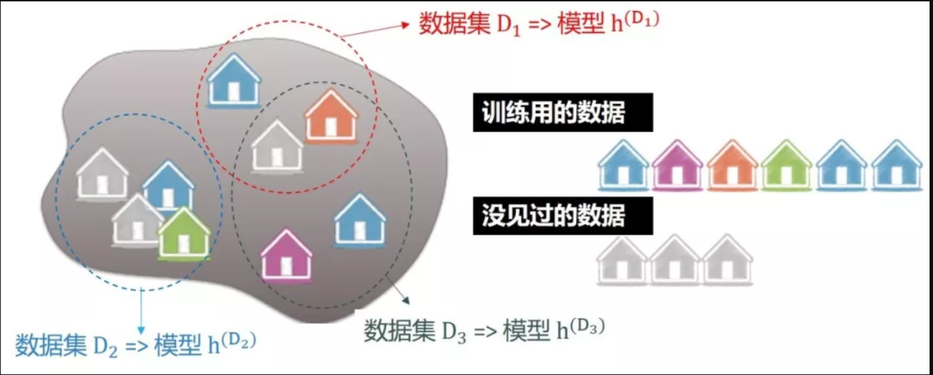
如图不同模型,给出不同的预测值,可以求出期望。
假设真实值为 g,每个预测值为 \(h^{D_i}\),预测值的期望为 \(f = E(h^{D})\)。
因此推导中的
\[\operatorname{Bias} = \sum(f - g)^2/n\] \[\operatorname{Variance} = \sum(f - h^{D})^2/n\]
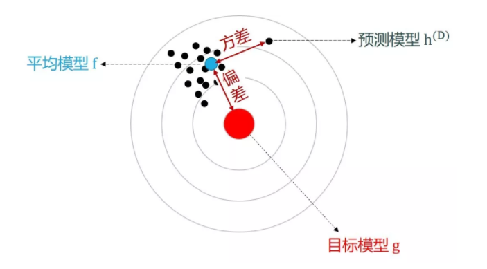
Figure 47.1: Bias 和 Variance 图像上的表达
目标模型可以说完美模型,那么就是真实值,因此可以说真实值和平均模型(训练集)的差异。 平均模型(训练集)和预测模型(预测集)的差异,也就是模型预测值的差异程度,真的是同一个样本的预测值,是多个模型给的。
实际过程中,
- 训练集上只有一个模型的话,这个模型就代表了\(f\),因此\(\operatorname{Bias} = \sum(f - g)^2/n\) 代表了训练集上的误差
- \(h^{D}\)代表了若干个开发集上的误差,因此\(\operatorname{Variance} = \sum(f - h^{D})^2/n\) 代表了开发集上的预测值差异,因为对应的真实值都相同,因此代表了训练集和开发集上误差的差异
因此
- bias 是训练集上 \(\hat y\) 和 \(y\) 的差异
\(\mathrm{{bias}_{train}}\),
- 同时也反映了\(\hat y\)和\(y\)两者 global mean 的差异,这里在 Mount and Zumel (2019a) 的模型校正问题上有所体现。
- 也反映 calibration curve 的差异,也就是各个 decile mean 的差异。
- variance 更突出泛化能力,是训练集和测试集上的差异,表现为 \(\mathrm{{bias}_{test}- {bias}_{train}}\)
47.2 推导
参考 www.statworx.com,假设
\[y_{i}=f\left(x_{i}\right)+\epsilon_{i}, \quad i=1, \ldots, n\]
因此
\[\begin{array}{l}{ M S E=n^{-1} \sum_{i=1}^{n}\left[\hat{f}\left(x_{i}\right)-f\left(x_{i}\right)\right]^{2} \\ M S E=n^{-1} \sum_{i=1}^{n}\left[\hat{f}\left(x_{i}\right)- E\left(\hat{f}\left(x_{i}\right)\right) + E\left(\hat{f}\left(x_{i}\right)\right) - f\left(x_{i}\right)\right]^{2} \\ M S E=n^{-1} \sum_{i=1}^{n}\left[\hat{f}\left(x_{i}\right)- E\left(\hat{f}\left(x_{i}\right)\right)\right]^{2} + n^{-1} \sum_{i=1}^{n}\left[E\left(\hat{f}\left(x_{i}\right)\right) - f\left(x_{i}\right)\right]^{2} \\ M S E=n^{-1} \sum_{i=1}^{n}\left[E\left(\hat{f}\left(x_{i}\right)\right)-f\left(x_{i}\right)\right]^{2}+n^{-1} \sum_{i=1}^{n} \operatorname{Var}\left(\hat{f}\left(x_{i}\right)\right)} \\ {M S E=\operatorname{Bias}^{2}+\text {Variance}}\end{array}\]
以上是 bias 和 variance 的推导。
47.3 过拟合和欠拟合图示
47.4 其他
47.4.1 生活的例子
机器学习算法与自然语言处理 (2018) 举例,用了一个学语言的例子。例如,如果你从小只学习了文言文。如果学习的特别认真,那么就过拟合了(overfitting),你太依赖自己的训练组, 然后你外出,跟人对话句句之乎者也,那么你的效果可能不好,这就是泛化能力不好(generalization)。 反之,你相信任何的语言源头都不够好,你不是特别相信,反正这种依赖原来训练组的行为,心里抵触,那么导致的结果就是,训练组和测试组的内在联系人为调控下降,因此欠拟合(underfitting)了,是泛化能力不好。 总之,最好的方法就是学习普通话,提高你的训练组。 另外,你到处游玩,只有文言文和普通话,肯定是不行的,不然你到成都的街头走一走,也很尴尬。 这个简单的例子,实现几个定义的理解。
- 过拟合,太依赖训练组。
- 欠拟合,不依赖训练组,一定程度上忽视训练组和测试组的内在联系。
一般地,过拟合的,都是高方差和低偏差的。
- 高方差,high variance,说明在训练组中,\(\hat y\)围绕\(\bar y\)的波动很大,类似于\(R^2\)的定义。
- 低偏差,low bias,对模型的假设违背的很少,必然啊,太依赖训练组,当然不会违背训练组训练出来的模型的假设。
相反,过拟合的,都是低方差和高偏差的。
- 低方差,说明在训练组中,\(\hat y\)围绕\(\bar y\)的波动很小,类似于\(R^2\)的定义。因为欠拟合忽略了不依赖训练组。
- 高偏差,对模型的假设违背的很搞,必然啊,不依赖训练组,当然违背训练组训练出来的模型的假设。
因此再浓缩,
- 过拟合 \(\to\) 依赖 \(\to\) \(Var(\hat y - \bar y)\)高,偏离假设小 \(\to\) 低bias
- 欠拟合 \(\to\) 不依赖 \(\to\) \(Var(\hat y - \bar y)\)低,偏离假设高 \(\to\) 高bias
过拟合学习了训练集自身的特点,比如训练集是叶子,有一部分锯齿的,预测叶子必须有锯齿; 欠拟合未学习好训练集自身的特点,比如训练集是叶子,绿色的,误以为绿色的都是叶子。 (周志华 2016)
47.4.2 特征变量太多\(\to\)过拟合
作为一个启发性例子,不妨假设 n=p=100。此时,即使这100个解释变量 x 与被解释变量 y 毫无关系(比如,相互独立),但将 y 对 x 作 OLS 回归,也能得到拟合优度 的完美拟合。这是因为,根据线性代数的知识,一个100维的向量组,其最大可能的秩为100。换言之,如果所有100个 x 向量均线性无关,则第101个向量(即 y)一定可以由这100个 x 向量所线性表出。 (陈强 2018b)
48 模型校正
48.1 介绍
样本迁移,会导致模型的预测值相对于真实值偏高或者偏低。 最常见的情况是
- 预测值的 global mean 和真实值的 global mean 不一致。
- 预测值的 decile mean 和真实值的 global decile 不一致,即使 lift 图是单调的。
通常我们会使用 calibration curve 来进行检验。
- Python 中
sklearn.calibration.calibration_curve函数会进行检验。 - R 中
add2evaluation::calibration_curve函数会进行检验。
Xgboost 中解决的办法是设置 basic_score=mean(y)(Mount and Zumel 2019c),这样的话至少
预测值的 global mean 和真实值的 global mean 不一致。
这个问题解决了。
但是 calibration curve 函数还是有偏移的情况。
通常是因为 nrounds 设置过小导致的,一般 20左右,最好>100。
因此这也是一种欠拟合的情况。
48.2 均值差异表现
48.3 相关文章阅读
In this note we have shown the consequences of different modeling decisions, in particular the trade-off between bias and relative error. (Mount and Zumel 2019b)
很显然,这里没有样本迁移 (bias) 的问题时,其实误差 (RMSE) 却很高。
we will show that common tree models are also non-calibrated, which means that despite their high accuracy on individual predictions. (Mount and Zumel 2019b) However, when making predictions on individuals, a biased model may be preferable; biased models may be more accurate, or make predictions with lower relative error than an unbiased model. For example, tree-based ensemble models tend to be highly accurate, and are often the modeling approach of choice for many machine learning applications. In this note, we will show that tree-based models are biased, or uncalibrated. This means they may not always represent the best bias/variance trade-off. (Mount and Zumel 2019a)
特别地,树模型也是有类似的问题。 一般来说,对用户层级的预测时,我们会多考虑 biased 模型,因为准确率更高,因此一直是一个 tradeoff 的问题。
A calibrated model is important in many applications, particularly when financial data is involved. (Mount and Zumel 2019a)
在当年的光伏发电比赛中,我们发现,一个光伏板普遍预测值高于真实值,这是属于模型没有校正 (uncalibrated) 的问题。
| education | income | pred_rf_raw |
|---|---|---|
| no high school diploma | 31883.18 | 41673.91 |
| Regular high school diploma | 38052.13 | 42491.11 |
| GED or alternative credential | 37273.30 | 43037.49 |
| some college credit, no degree | 42991.09 | 44547.89 |
| Associate’s degree | 47759.61 | 46815.79 |
| Bachelor’s degree | 65668.51 | 63474.48 |
| Master’s degree | 79225.87 | 69953.53 |
| Professional degree | 97772.60 | 76861.44 |
| Doctorate degree | 91214.55 | 75940.24 |
Note that the rollups of the predictions from the two ensemble models don’t match the true rollups, even on the training data. (Mount and Zumel 2019a)
就连训练集在树模型情况下也有样本迁移的情况。
However, even these more accurate ensemble models can be biased, so they are not guaranteed to estimate important aggregates (grouped sums or conditional means) correctly. (Mount and Zumel 2019a)
因此在做渠道价值相关模型时,把个人聚合到渠道层面时,需要做校正处理 (calibrating)。
The issue is hidden in the usual value of the “learning rate” eta. In gradient boosting we fit sub-models (in this case regression trees), and then use a linear combination of the sub-models predictions as our overall model. However: eta defaults to 0.3 (ref), which roughly means each sub-model is used to move about 30% of the way from the current estimate to the suggested next estimate. Thus with a small number of trees the model deliberately can’t model the unconditional average as it hasn’t been allowed to fully use the sum-model estimates. (Mount and Zumel 2019c)
学习率衡量了移动的步子,这个解释很有意思。
就是学习率和迭代次数的造成的影响,之前我也发现了。
48.4 解决办法
48.4.1 base score
Or we can fix this by returning to the documentation, and noticing the somewhat odd parameter “base_score”. (Mount and Zumel 2019c) Why does this issue live on? Because, as the documentation says, it rarely matters in practice. However it may be a good practice to try setting base_score = mean(d$y) (especially if your model is having problems and you are seeing a small number of trees in your xgboost model). (Mount and Zumel 2019c)
base_score = mean(d$y) 这是一个很好的 sense,减少 variance。
48.4.2 base_score 算法位置
\[\text {Sigmoid }\left(\sum(\text {TreeLeaves})+\text {logit}(\text {basescore})\right)\]
参考dmlc/xgboost #4682 和 discuss.xgboost.ai
在工程上,
- 如果是默认 0.5,那么是自动加上的
- 如果是其他的,就没有自动加上去,而需要自己加上去。
xgb_pred_fun <- function(tree_leaves, base_score = 0.5){1/(1 + exp(-(sum(tree_leaves) + base_score)))}
xgb_pred_fun(
    tree_leaves = c(0.009677419,-0.034775745,0.098971337,0.071213789),
    base_score = 0.5
)
## [1] 0.655902448.4.3 more nrounds
We can fix this by running xgboost closer to how we would see it run in production (which was in fact how Nina ran it in the first place!). Run for a larger number of rounds, and determine the number of rounds by cross-validation. (Mount and Zumel 2019c)
base_score只能解决均值的差异,但是对于 calibration curve 上的差异,还是需要通过提高 nrounds 来完成。
48.4.4 Stacking
you can think of this polishing procedure as being a form of stacking, where some of the sub-learners are simply single variables. (Mount and Zumel 2019c)
这是一个类似于 stacking 的方法。
This method is ad-hoc, and may be somewhat brittle. In addition, it requires that the data scientist knows ahead of time which rollups will be desired in the future. However, if you find yourself in a situation where you must balance accurate individual prediction with accurate aggregate estimates, this may be a useful trick to have in your data science toolbox. (Mount and Zumel 2019c)
当要对某个变量进行 groupby 拿到 agg 值。由于样本迁移的问题(用树模型就是有),汇总值有问题,这个时候可以再对
\[y - \hat y \sim \text{cate}\]
用这个差异再加在 \(\hat y\) 上即可(Mount and Zumel 2019c)。
49 逻辑回归
\[\log(\frac{p}{1-p}) = \beta_0 + \beta_1 x + \mu\]
等价于
\[p = \frac{1}{1+e^{-(\beta_0 + \beta_1 x + \mu)}}\]
一般逻辑回归的预测值为
\[\hat p = \frac{1}{1+e^{-(\hat \beta_0 + \hat \beta_1 x)}}\]
因此 \(\hat p\) 怎么定义,就很容易理解了。
WOE 等归在 x 这里。
50 MLE
逻辑回归的是通过 MLE 实现的。
\[\log \left(\prod_{i=1}^{N} \operatorname{Pr}\left(X_{i}=x_{i}\right)\right)=\sum_{i=1}^{N} \log \left(\operatorname{Pr}\left(X_{i}=x_{i}\right)\right)\]
假设每个点的概率最大化的情况去看。
one thus needs to assume a certain probability distribution, and then look for the parameters that maximize the likelihood that this distribution generated the observed data (Rodrigues 2019) First of all, let’s assume that each observation from your dataset not only was generated from the same distribution, but that each observation is also independent from each other. For instance, if in your sample you have data on people’s wages and socio-economic background, it is safe to assume, under certain circumstances, that the observations are independent. (Rodrigues 2019)
假设一个分布,然后通过迭代,最拟合它。 这里的样本假设是独立的,而且是同分布(因此为什么会有图神经网络,就是解决这种不独立的情况)。
Maximum likelihood estimation is a very useful technique to fit a model to data used a lot in econometrics and other sciences, but seems, at least to my knowledge, to not be so well known by machine learning practitioners (Rodrigues 2019)
因为 MLE 理解起来比较不直接,因此 参考 Rodrigues (2019) 这里仿真做一个实验。
x1 <- rnorm(size)
x2 <- rnorm(size)
x3 <- rnorm(size)
mu <- rnorm(size)
y <- 1.5 + 2*x1 + 3*x2 + 4*x3 + mu

df <- data.frame(y, iota = 1, x1, x2, x3)

df
loglik_linmod <- function(parameters, x_data){
sum_log_likelihood <- x_data %>%
mutate(log_likelihood =
dnorm(y,
mean = iota*parameters[1] + x1*parameters[2] + x2*parameters[3] + x3*parameters[4],
sd = parameters[5],
log = TRUE)) %>%
summarise(sum(log_likelihood))
-1 * sum_log_likelihood
}## $par
## [1] 1.515660 1.969141 3.012765 3.920610 1.057969
##
## $value
## [1] 147.512
##
## $counts
## function gradient
## 502 NA
##
## $convergence
## [1] 1
##
## $message
## NULL注意最后的 beta 趋近于 1.5,2,3,4,mu sd 趋近于 1。
51 先做端到端的工作
先做端到端的工作,然后一次改进一件事。 从可能有效的最简单的事情开始,然后部署它。你会从中学到很多。过程中任何阶段的额外复杂性都会改进研究论文中的模型,但很少会改进现实世界中的模型。每一个额外的复杂性都需要验证。 从可能有效的最简单的事情开始,然后部署它。 将一些东西交到最终用户手中,可以帮助你尽早了解模型可能工作得有多好,并且它可能会带来一些关键问题,比如模型正在优化的内容与最终用户想要的内容之间的分歧。它还可能使你重新评估你正在收集的训练数据的类型。最好能尽快发现这些问题。 (Biewald 2020)
了解模型的最后实用性和落地情况。
52 树模型不必分箱
分箱作用本身就是为了处理极值问题,线性模型LR这种才有影响。树模型本身每个 split 都是根据 gain、similarity score 这类去切,本身已经处理分箱问题,根本没必要再分箱。 分箱是为了处理异常值,但是本身树模型就是处理异常值的,在 y 的维度和 x 维度上都有。
53 正则化处理的地方

Figure 53.1: 越靠近 output 效果越好。
54 加载带有自定义损失函数的模型
55 python 分类变量处理
pandas.Series.cat.codes 得到分类的 index,再注意,对于 keras.utils.to_categorical这些函数,都需要 index=0的,需要这样的操作。
robust 的写法是强写 astype('category'),因为这个需要先转换从非 int。
56 AttributeError: ‘Model’ object has no attribute ‘predict_classes’
参考 https://blog.csdn.net/zds13257177985/article/details/80638384
57 keras regression rsquare negative
欠拟合,相当于 embedding 一开始的都没有梯度下降足够!放到 train_model 里面 因为词向量没有训练好,所以才会那么差。
参考文献
Bennett, Mark J., and Dirk L. Hugen. 2016. Financial Analytics with R: Building a Laptop Laboratory for Data Science. Cambridge University Press. https://doi.org/10.1017/CBO9781316584460.
Biewald, Lukas. 2020. “为什么机器学习项目非常难管理?.” AI公园. 2020. https://mp.weixin.qq.com/s/hxTYnLMrmmXhsTCcc_FREg.
Box, G. E. P., and D. R. Cox. 1964. “An Analysis of Transformations.” Journal of the Royal Statistical Society 26 (2): 211–52.
Carolin, Strobl, Boulesteix Anne-Laure, Kneib Thomas, Augustin Thomas, and Zeileis Achim. 2008. “Conditional Variable Importance for Random Forests.” Bmc Bioinformatics 9 (1): 1–11.
Chan, Kung-Sik, and Brian Ripley. 2012. TSA: Time Series Analysis. https://CRAN.R-project.org/package=TSA.
Chapman, Christopher N., and Mc Donnell Feit. 2015. R for Marketing Research and Analytics. Springer International Publishing.
Chen, Tianqi. 2016. “Why Is Xgboost Given so Much Less Attention Than Deep Learning Despite Its Ubiquity in Winning Kaggle Solutions?” 2016. https://www.quora.com/Why-is-xgboost-given-so-much-less-attention-than-deep-learning-despite-its-ubiquity-in-winning-Kaggle-solutions/answer/Tianqi-Chen-1.
Chen, Xi, and Hemant Ishwaran. 2012. “Random Forests for Genomic Data Analysis.” Genomics 99 (6): 323–29. https://doi.org/https://doi.org/10.1016/j.ygeno.2012.04.003.
DiFranco, Tony. 2016. “Tweedie Regression Demo in R.” 2016. https://github.com/dmlc/xgboost/blob/master/R-package/demo/tweedie_regression.R.
DMLC. 2018. “XGBoost Parameters: Parameters for Tweedie Regression.” 2018. https://xgboost.readthedocs.io/en/latest/parameter.html#parameters-for-tweedie-regression-objective-reg-tweedie.
George, Nathan. 2018. “Machine Learning for Finance in Python.” DataCamp. 2018. https://www.datacamp.com/courses/machine-learning-for-finance-in-python.
Guan, Xiaowei, Mark R Chance, and Jill S Barnholtzsloan. 2012. “Splitting Random Forest (Srf) for Determining Compact Sets of Genes That Distinguish Between Cancer Subtypes.” Journal of Clinical Bioinformatics 2 (1): 13.
Jamshidi, Arash. 2018. “Strings as Features in Decision Tree/Random Forest.” 2018. https://datascience.stackexchange.com/questions/5226/strings-as-features-in-decision-tree-random-forest.
jlhoward. 2017. “R Codes for Tweedie Compound Poisson Gamma.” 2017. https://stackoverflow.com/questions/21807118/r-codes-for-tweedie-compound-poisson-gamma.
Johnson, Paul E. 2014. “GLM with a Gamma-Distributed Dependent Variable.” 2014. http://pj.freefaculty.org/guides/stat/Regression-GLM/Gamma/GammaGLM-01.pdf.
Kabacoff, Robert I. 2017. “Generalized Linear Models.” 2017. https://www.statmethods.net/advstats/glm.html.
LaBarr, Aric. 2018. “Forecasting Product Demand in R.” DataCamp. 2018. https://www.datacamp.com/courses/forecasting-product-demand-in-r.
Lantz, Brett. 2017. “Supervised Learning in R: Classification.” 2017. https://www.datacamp.com/courses/supervised-learning-in-r-classification.
Lee, Myoung-jae. 2014. Micro-Econometrics: Methods of Moments and Limited Dependent Variables. Springer.
Li, Jiaxiang. 2018a. “Choosing Between Lm and Glm for a Log-Transformed Response Variable.” 2018. https://stats.stackexchange.com/questions/43930/choosing-between-lm-and-glm-for-a-log-transformed-response-variable/349552#349552.
———. 2018b. “How Do I Predict New Data’s Cluster After Clustering Training Data?” Stack Overflow. 2018. https://stackoverflow.com/questions/21064315/how-do-i-predict-new-datas-cluster-after-clustering-training-data/52184016#52184016.
Masterov, Dimitriy V. 2014. “Data Preparation for Gradient Boosting with Xgboost in Python.” 2014. https://stats.stackexchange.com/questions/96972/how-to-interpret-parameters-in-glm-with-family-gamma.
Mayank. 2016. “Hclust() in R on Large Datasets.” Stack Overflow. 2016. https://stackoverflow.com/questions/40989003/hclust-in-r-on-large-datasets?noredirect=1.
Mount, John, and Nina Zumel. 2019a. “Common Ensemble Models Can Be Biased.” Win-Vector LLC. 2019. http://www.win-vector.com/blog/2019/07/common-ensemble-models-can-be-biased/.
———. 2019b. “Link Functions Versus Data Transforms.” Win-Vector LLC. 2019. http://www.win-vector.com/blog/2019/07/link-functions-versus-data-transforms/.
———. 2019c. “Some Details on Running Xgboost.” Win-Vector LLC. 2019. http://www.win-vector.com/blog/2019/07/some-details-on-running-xgboost/.
Ng, Andrew. 2018. “Machine Learning Yearning.” 2018. http://www.mlyearning.org/.
Prabhakaran, Selva. 2017. “Association Mining (Market Basket Analysis).” r-statistics.co. 2017. http://r-statistics.co/Association-Mining-With-R.html.
Prophet60091. 2014. “Limits to Tree-Based Ensemble Methods in Small N, Large P Problems?” Stack Exchange. 2014. https://stats.stackexchange.com/q/128758.
Python Software Foundation. 2018. “LightGBM Python Package.” 2018. https://pypi.org/project/lightgbm/.
Raad. 2015. “ARIMA Forecasting with auto.Arima() and Xreg.” 2015. https://stackoverflow.com/questions/34249477/arima-forecasting-with-auto-arima-and-xreg?rq=1.
Revelle, William. 2011. “Q and R Mode in Principal Component Analysis: Applied Multivariate Statistics – Spring 2012.” 2011. https://stat.ethz.ch/pipermail/r-help/2011-September/289101.html.
Rodrigues, Bruno. 2019. “Split-Apply-Combine for Maximum Likelihood Estimation of a Linear Model.” Econometrics and Free Software. 2019. https://www.brodrigues.co/blog/2019-10-05-parallel_maxlik/.
Rodríguez, Germán. 2007. “Lecture Notes on Generalized Linear Models: Chapter 4 Poisson Models for Count Data.” 2007. http://data.princeton.edu/wws509/notes/c4.pdf.
Sanchez, Benoit. 2017. “Difference Between Logit and Probit Models.” 2017. https://stats.stackexchange.com/q/30909.
Sandhu, Sandeep S. 2016. “How Do I Interpret the Output of Xgboost Importance?” 2016. https://datascience.stackexchange.com/questions/12318/how-do-i-interpret-the-output-of-xgboost-importance.
Shukla, Rishabh. 2015. “L1 Vs. L2 Loss Function.” 2015. http://rishy.github.io/ml/2015/07/28/l1-vs-l2-loss/.
Silge, Julia. 2018. “Supervised Learning in R: Case Studies.” 2018. https://campus.datacamp.com/courses/supervised-learning-in-r-case-studies/get-out-the-vote?ex=9.
Stack Exchange. 2012a. “Choosing Between Lm and Glm for a Log-Transformed Response Variable.” Cross Validated. https://stats.stackexchange.com/q/43930.
———. 2012b. “Difference Between Logit and Probit Models.” 2012. https://stats.stackexchange.com/q/30909.
———. 2013a. “Confusion Related to Which Transformation to Use.” Cross Validated. https://stats.stackexchange.com/q/67505.
———. 2013b. “When to Use Gamma Glms?” Cross Validated. https://stats.stackexchange.com/q/67550.
Strobl, Carolin, Anne Laure Boulesteix, Thomas Kneib, Thomas Augustin, and Achim Zeileis. 2008. “Conditional Variable Importance for Random Forests.” Bmc Bioinformatics 9 (1): 307–7.
Strobl, Carolin, Torsten Hothorn, and Achim Zeileis. 2009. “Party on! A New, Conditional Variable Importance Measure for Random Forests Available in the Party Package.” Christian Century 1 (2): 14–17.
Strobl, Carolin, and Achim Zeileis. 2008a. “Danger: High Power! – Exploring the Statistical Properties of a Test for Random Forest Variable Importance.”
———. 2008b. “Why and How to Use Random Forest Variable Importance Measures (and How You Shouldn’t).” Dortmund: useR! 2008. http://www.statistik.uni-dortmund.de/useR-2008/slides/Strobl+Zeileis.pdf.
Tianqi Chen, Michaël Benesty, Tong He. 2018. “Understand Your Dataset with Xgboost.” 2018. https://cran.r-project.org/web/packages/xgboost/vignettes/discoverYourData.html#numeric-v.s.-categorical-variables.
Todorov, Kaloyan. 2013. “How Do I Create a Copy of a Data Frame in R.” 2013. https://stackoverflow.com/questions/18346719/how-to-deal-with-log-of-zero-in-r-in-image-plot/18347145#18347145.
Warden, Pete. 2018. “Why You Need to Improve Your Training Data, and How to Do It.” PETE WARDEN’S BLOG. 2018. https://petewarden.com/2018/05/28/why-you-need-to-improve-your-training-data-and-how-to-do-it/.
Wikipedia contributors. 2018a. “Probit Model — Wikipedia, the Free Encyclopedia.” https://en.wikipedia.org/w/index.php?title=Probit_model&oldid=841156213.
———. 2018b. “Variance Inflation Factor — Wikipedia, the Free Encyclopedia.” https://en.wikipedia.org/w/index.php?title=Variance_inflation_factor&oldid=850910818.
Yee, Thomas W. 2015. Vector Generalized Linear and Additive Models: With an Implementation in R. Springer Publishing Company, Incorporated.
Zherebetskyy, Danylo. 2017. “How to Handle Categorical Features for Decision Tree, Random Forest in Spark Ml?” 2017. https://stackoverflow.com/questions/44959122/how-to-handle-categorical-features-for-decision-tree-random-forest-in-spark-ml.
周志华. 2016. 机器学习: Machine Learning. 清华大学出版社.
圣蕾. 2018. “吴恩达教你应用机器学习技巧.” 2018. https://mp.weixin.qq.com/s/dhroDk4QbIUV2dQxxzNQjA.
姚岑卓. 2017. “在统计学中为什么要对变量取对数.” 2017. https://www.zhihu.com/question/22012482/answer/21315349.
张建军. 2018. “通俗聊聊损失函数中的均方误差以及平方误差.” 2018. https://mp.weixin.qq.com/s/YOdmv88koSHx5AMMEQZGgg.
慧航. 2014. “在统计学中为什么要对变量取对数.” 2014. https://www.zhihu.com/question/22012482/answer/34795487.
机器学习算法与自然语言处理. 2018. “一文区分什么是「过拟合」和「欠拟合」?.” 2018. https://mp.weixin.qq.com/s/_V1Yno4FzhGdGqr6JPscpw.
李家伟. 2017. “泊松分布 (Poisson Distributions) 的推导.” 2017. https://zhuanlan.zhihu.com/p/26263743.
杜雨. 2018. “杜雨.” 2018. https://mp.weixin.qq.com/s/U0hqJ-ny3fPTXSP2J1BOLg.
王圣元. 2018a. “解读吴恩达新书的全球第一帖 (上).” 2018. https://mp.weixin.qq.com/s/5A6DadzIHvN9Z7UVTUrrzw.
———. 2018b. “解读吴恩达新书的全球第一帖 (中).” 2018. https://mp.weixin.qq.com/s/w7j1B55tKoy-H3Lau78G-g.
申利彬, and 丁楠雅. 2018. “如何改善你的训练数据集?.” 大数据文摘. 2018. https://mp.weixin.qq.com/s/lMU6_ywQqneyunqEV6uDiA.
陈强. 2018a. “为何你还没理解主成分分析.” 2018. https://mp.weixin.qq.com/s/_2SirRp3DGbbLHHHV4xqoA.
———. 2018b. “当计量经济学遭遇机器学习(三):高维回归之岭回归.” 2018. https://mp.weixin.qq.com/s/YIFljbIp9Wr3kodrDjXpLA.
这里的开发集就是验证集,validation set↩︎
Todorov (2013) 也给出另一种方式,如果分布中有0的情况,为了处理右偏的情况,可以使用 \[\sqrt[n]{x}, n>1\] 关于n次根的效果,时常会高于log变换,详见 22.3↩︎
这里肯定要做降维。↩︎
由泰勒公式, \[\begin{alignat}{2} \log(x+1) &= \sum_{i=1}^{\infty}\frac{(-1)^{n=1}}{n}x^n = x - \frac{x^2}{2} + \frac{x^3}{3} - \cdots \\ &\approx x \end{alignat}\]↩︎
我们会发现这个和一般的损失函数不同,例如OLS的损失函数为 \[L = \sum_{i=1}^n (y- \hat y)^2\] 然而最大似然估计方程前有一个负数,这是因为 \[h_{\theta}(x) \in (0,1) \to \begin{cases} \log (h_{\theta}(x)) < 0 \\ 1- \log (h_{\theta}(x)) < 0\\ \end{cases}\] 因此当加上\(-1\)时,条件转化为标准损失函数求解的情况,并使用梯度下降进行计算。 \[\beta := \beta + \alpha - \frac{\partial \log(L(\beta))}{\partial \beta}\] 详见逻辑回归↩︎
“A common rule of thumb is that V IF > 5.0 indicates the need to mitigate collinearity.”(Chapman and Feit 2015,Chapter 9.1.2) 因此cutoff没有一个唯一的标准。↩︎